Review of data processing of functional optical microscopy for neuroscience

Abstract

Functional optical imaging in neuroscience is rapidly growing with the development of optical systems and fluorescence indicators. To realize the potential of these massive spatiotemporal datasets for relating neuronal activity to behavior and stimuli and uncovering local circuits in the brain, accurate automated processing is increasingly essential. We cover recent computational developments in the full data processing pipeline of functional optical microscopy for neuroscience data and discuss ongoing and emerging challenges.

Keywords: calcium imaging; data analysis; fluorescence microscopy; functional imaging.

Fig. 1

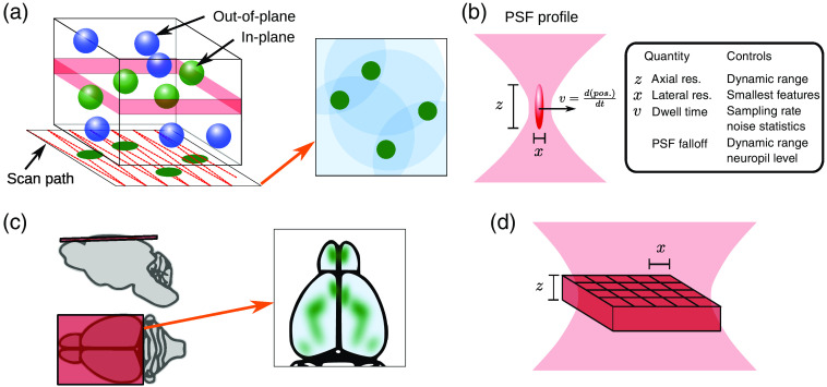
Optical imaging basics. (a) Laser scanning microscopy (e.g., two-photon microscopy) focuses the laser on a point inside the tissue, sequentially illuminating a chosen plane. Neurons intersecting the plane show up in the rendered images, whereas out-of-plane neurons accumulate as background, and combined nonsomatic activity (e.g., smaller dendritic and axonal components) as neuropil. (b) Choices in the optical illumination impact image properties. The image resolution is defined by the PSF, which is determined by microscope optics and optical properties of the sample. The dwell time controls the time spent at each location and is related to the scanning speed, i.e., the framerate, and can influence the number of photons collected per pixel and thus the signal strength. In laser scanning microscopy, these, in combination with scanning and laser technology, the image size, resolution, framerate, and noise characteristics of the image are determined. (c) Widefield imaging simultaneously illuminates the entire cortical surface plane, capturing dynamics across multiple brain areas. (d) In widefield imaging, camera characteristics primarily determine the image acquisition size and rate. The optical resolution for widefield imaging is strongly limited by microscope optics and optical aberrations from the sample.

Fig. 2

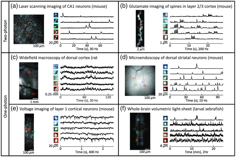
Examples of functional microscopy data. Functional microscopy data obtained via different modalities, at different scales, and in different animal models expressing different indicators can take on a diversity of signal characteristics. Shown are six examples spanning a range of datasets. (a) Laser scanning two-photon calcium imaging (GCaMP5) in mouse hippocampus. (b) Glutamate (iGluSnFR3.v857) spine imaging using laser-scanning two-photon microscopy in layer two-third mouse cortex. (c) One-photon widefield calcium (GCaMP6f) imaging of rat dorsal cortex using a head-mounted macroscope. (d) One-photon calcium imaging using a head-mounted microendoscope in mouse striatum. (e) One-photon voltage imaging (Voltron525-ST) in layer 1 of mouse cortex. (f) Whole-brain light-sheet calcium imaging (GCaMP6f) in larval zebrafish. Only one of 29 imaging planes each recorded at 2 Hz is depicted here. Note that the spatial and temporal statistics range dramatically across domains, requiring flexible data processing approaches.

Fig. 3

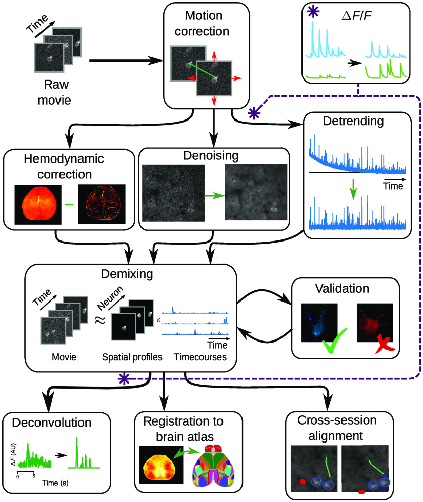
The optical imaging pipeline, expanded. The first step in analyzing fluorescence microscopy data is to correct any motion, reducing interframe misalignment. Between motion correction and demixing (i.e., cell-finding), steps to remove imaging noise and confounding factors are taken. Specific steps include de-trending to remove photobleaching, denoising to increase SNR, and hemodynamic correction in widefield data. The core pipeline stage of focus is demixing or identification of individual fluorescing components. Demixing should always be paired with some sort of validation on the output to prevent artifacts and other errors. The output of the demixing can be used to infer firing events (in single-cell resolution imaging), align multiple imaging sessions, or register to a global brain atlas (in widefield data). One important step: the $\mathrm{\Delta }F/F$ calculation, which normalized fluorescence traces to their baseline, can be computed before or after demixing.

Fig. 4

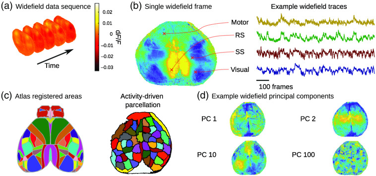
Widefield imaging. (a) Imaging frames of widefield signal. (b) Left—a single frame, red “$x$” correspond to motor, retrosplenial (RS), somatosensory (SS), and visual cortices, right—time-traces of the corresponding locations. (c) Left—anatomical atlas CCFv3, right—functional parcellation by LSSC. (d) Spatial components derived by SVD. Data from Ref. .

Fig. 5

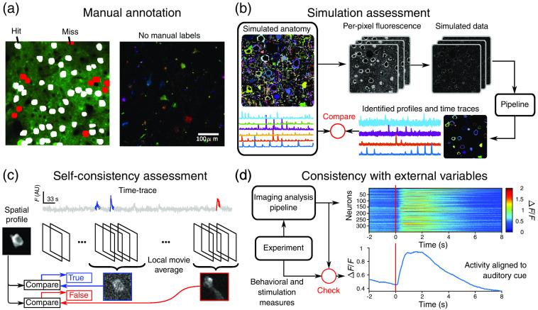
Assessing optical imaging analysis outputs. (a) Manual annotation, e.g., the NeuroFinder benchmark dataset (example shown here), can help detect true detections (white) and missed cells (red), as compared with a labeling of the spatial area imaged (right). Manual annotation, however, does not provide information on cells that do not match any of the manual annotations (left). (b) Simulation-based assessment uses in silico simulations of activity and anatomy to create faux fluorescence microscopy data. The outputs of an analysis pipeline using the data can be compared with the simulated ground truth. (c) Self-consistency measures use the global demixed components and analyze local space-time extents of the movie to check if the spatial and temporal components still describe the data well. For example, is activity erroneously attributed to a found cell. (d) Consistency with external variables examines if expected gross behavior of the imaged neural populations match behavioral or stimulation events corecorded with the fluorescence video. For example, shown here are neurons in motor cortex responding to a motion made by a mouse responding to an auditory cue.