Evaluating the Performance of Using Low-Cost Sensors to Calibrate for Cross-Sensitivities in a Multipollutant Network

Abstract

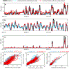
As part of our low-cost sensor network, we colocated multipollutant monitors containing sensors for particulate matter, carbon monoxide, ozone, nitrogen dioxide, and nitrogen monoxide at a reference field site in Baltimore, MD, for 1 year. The first 6 months were used for training multiple regression models, and the second 6 months were used to evaluate the models. The models produced accurate hourly concentrations for all sensors except ozone, which likely requires nonlinear methods to capture peak summer concentrations. The models for all five pollutants produced high Pearson correlation coefficients (r > 0.85), and the hourly averaged calibrated sensor and reference concentrations from the evaluation period were within 3-12%. Each sensor required a distinct set of predictors to achieve the lowest possible root-mean-square error (RMSE). All five sensors responded to environmental factors, and three sensors exhibited cross-sensitives to another air pollutant. We compared the RMSE from models (NO₂, O₃, and NO) that used colocated regulatory instruments and colocated sensors as predictors to address the cross-sensitivities to another gas, and the corresponding model RMSEs for the three gas models were all within 0.5 ppb. This indicates that low-cost sensor networks can yield useable data if the monitoring package is designed to comeasure key predictors. This is key for the utilization of low-cost sensors by diverse audiences since this does not require continual access to regulatory grade instruments.

Keywords: AlphaSense; Plantower; calibration; low-cost sensor; regression models.

Figure 1.

(A–D) Time series of the hourly averaged reference (black) and PM_2.5 and CO sensor data from the training (uncalibrated data displayed in red; left column) and evaluation (calibrated displayed in blue; right column) periods. The uncorrected CO sensor (in mV) is the difference between the working electrode and the auxiliary electrode. (E,F) Scatterplots of the sensor vs reference data from the two periods. Note: the raw sensor values shown here are specific to this individual sensor and not representative of all sensors of the same type, but the responses (e.g., reducing output because of exposure to a pollutant or changing environmental conditions) should be similar across different sensor of the same type. The linear fits for the evaluation periods are displayed.

Figure 2.

Time series of the hourly averaged reference data (black) and NO₂, O₃, and NO sensor data from the training (uncalibrated data shown in red; left column) and evaluation (calibrated shown in blue; right column) periods. The uncorrected NO₂ and NO sensors (in mV) are the difference between the working electrode and the auxiliary electrode.

Figure 3.

Calibration model results using either hourly reference data or colocated sensors as predictors to correct from cross-sensitive pollutants for (A) O₃, (B) NO₂, and (C) NO sensors, shown in greater detail for September 2019. The blue line was calculated using reference data for the predictors needed in the model (same as in Figure 2), and the red line was calculated by using data from other sensors colocated in the box. (D–F) Scatterplots of the model results and the reference data from the full evaluation period. The linear fits for the evaluation periods are displayed.

References

-
- Tan B Laboratory Evaluation of Low to Medium Cost Particle Sensors. MS Thesis, University of Waterloo, 2017.
- Ikram J; Tahir A; Kazmi H; Khan Z; Javed R; Masood U View: implementing low cost air quality monitoring solution for urban areas. Environ. Syst. Res 2012, 1, 10.
- Mead MI; Popoola OAM; Stewart GB; Landshoff P; Calleja M; Hayes M; Baldovi JJ; McLeod MW; Hodgson TF; Dicks J; Lewis A; Cohen J; Baron R; Saffell JR; Jones RL The use of electrochemical sensors for monitoring urban air quality in low-cost, high-density networks. Atmos. Environ 2013, 70, 186–203.
Grants and funding
LinkOut - more resources
Full Text Sources
Research Materials