The impact of sparsity in low-rank recurrent neural networks

Abstract

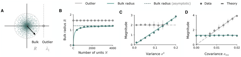
Neural population dynamics are often highly coordinated, allowing task-related computations to be understood as neural trajectories through low-dimensional subspaces. How the network connectivity and input structure give rise to such activity can be investigated with the aid of low-rank recurrent neural networks, a recently-developed class of computational models which offer a rich theoretical framework linking the underlying connectivity structure to emergent low-dimensional dynamics. This framework has so far relied on the assumption of all-to-all connectivity, yet cortical networks are known to be highly sparse. Here we investigate the dynamics of low-rank recurrent networks in which the connections are randomly sparsified, which makes the network connectivity formally full-rank. We first analyse the impact of sparsity on the eigenvalue spectrum of low-rank connectivity matrices, and use this to examine the implications for the dynamics. We find that in the presence of sparsity, the eigenspectra in the complex plane consist of a continuous bulk and isolated outliers, a form analogous to the eigenspectra of connectivity matrices composed of a low-rank and a full-rank random component. This analogy allows us to characterise distinct dynamical regimes of the sparsified low-rank network as a function of key network parameters. Altogether, we find that the low-dimensional dynamics induced by low-rank connectivity structure are preserved even at high levels of sparsity, and can therefore support rich and robust computations even in networks sparsified to a biologically-realistic extent.

Fig 1. Influence of sparsity on the eigenspectra of full-rank networks.

A: Illustration of how sparsity is imposed in the connectivity matrix, where the degree of sparsity is s = 0.5. B: Complex eigenspectra of full-rank, Gaussian connectivity matrices of finite size (N = 300, g = 1) in the dense case (left) and with a sparsity of 0.5 (right). The dashed line plots the unit circle. C, D, E: Reduction of spectral radius R as a function of sparsity in a full-rank matrix J constructed as in (Eq 2) with connection strength g = 1. In C, sparsity is imposed as a fraction of total connections removed (N = 1000). In D and E sparsity is imposed by fixing the number of outgoing connections to C = 200 and increasing N. Dots: mean empirical spectral radius, measured as the largest absolute value of all eigenvalues, over 50 instances. Solid lines: theoretical prediction (Eq (6)).

Fig 2. Influence of sparsity on the eigenspectra of rank-one networks.

A: Eigenspectra of rank-one connectivity matrices of finite size, in the dense case (left) and under a sparsity of 0.5 (right). The matrix P is constructed as in (Eq 3), with parameters σ² = 16, σ_mn = 1.44 and N = 300. Under sparsity, the outlier (gold) is reduced and the bulk distribution (brown) emerges. The dashed line plots the unit circle. B, C: Impact of sparsity on two key features of the eigenspectrum of finite-size rank-one networks: B, the outlier λ₁, and C, the spectral radius of the bulk distribution. The outlier is eventually reduced below the instability boundary of λ₁ = 1, dashed line. Sparsity is imposed as a fraction of total connections removed; σ² = 16, σ_mn = 4 and N = 1000. D: Same as in C but for sparsity imposed by fixing C = 200 non-zero connections and increasing N; bulk radius is plotted as a function of N. Dots: empirical measurements of outlier and bulk radius. Solid lines: theoretical prediction (Eq (9)).

Fig 3. Key features of rank-one eigenspectrum become independent of N in the high sparsity limit.

A: Illustration of the spectral radius R of the bulk distribution induced by sparsity, and the outlier λ₁ inherited from the rank-one structure. Dots: eigenvalues of matrix. Dashed lines: theoretical predictions, with C = 200, N = 2000, σ² = 0.09, and σ_mn = 0.008. B: Bulk radius (Eq 14) as a function of sparsity imposed by fixing C = 200 and increasing N, for the rescaled matrix P_ij = m_in_j with σ² = 0.09 and σ_mn = 0.008. The outlier Cσ_mn is now independent of N. The bulk radius converges towards $\sqrt{C}{\sigma }^2$ (dashed line) as sparsity increases. C: Outlier and bulk radius as a function of the variance of the connectivity vectors, while the covariance is fixed (σ_mn = 0.01). D: Outlier and bulk radius as a function of the covariance σ_mn, while the variance is fixed (σ² = 0.09). Empirical values are displayed as mean (dots) and standard deviation (bars, 10 repeats) of the eigenvalue with largest absolute magnitude (bulk) and real part (outlier), while the outlier is still distinguished from the bulk. When the outlier is smaller than the bulk, its location cannot be measured empirically. Lines: theoretical predictions at empirically measurable (solid) and unmeasurable (dashed) locations. Parameters: C = 200, N = 1200, resulting in s = 0.8.

Fig 4. Impact of sparsity on input-driven dynamics.

Network responses to a step input current along a random vector I. A-C: network consists of a dense rank-one component $\frac{1}{N}{m}_i{n}_j$ and a full-rank, Gaussian component of variance g²/N; the random strength g is progressively increased from zero to one, in order to increase the radius of the eigenvalue disk from zero to one. D-F: network consists only of rank-one component P_ij = m_in_j; the sparsity is progressively increased by decreasing the number of non-zero connections C. Parameters are chosen such that the radius of the eigenvalue bulk also spans the range [0, 1) as sparsity is modulated (σ² = 0.043). The outlier is fixed at zero (σ_mn = 0). The input vector I partially overlaps with n (σ_nI = 0.2). A, D: Temporal dynamics of the network during step input (A: g = 0.8; D: s = 0.8). Top: samples of input timeseries u(t)I_i. Bottom: samples of network activations x_i(t). B, E: Left: input-driven population trajectories projected onto the plane defined by the right connectivity vector m and input vector I, as random strength (resp. sparsity) is progressively increased. Right: principal component analysis (PCA) of each trajectory, showing the fraction of variance explained by the first three components (upper panels) and the correlation between first three principal components and the vectors I and m (lower panels). Examples are shown for both low and high random strength (resp. sparsity). C, F: Top: Dimensionality of network trajectories quantified by the participation ratio ${\left({\sum }_i{\lambda }_i\right)}^2/\left({\sum }_i{\lambda }_i^2\right)$, where λ_i are the eigenvalues of the covariance matrix of activations. Bottom: Projection of network activation x onto the right connectivity vector m (the latent variable κ_r). The analytical radius of the corresponding eigenvalue disk is also shown in grey. For comparison, we also plot the dimensionality of Gaussian network trajectories corresponding to values of g equal to the radius of the sparse networks (red curve). The mean value for both dimensionality and projections is taken over 50 simulations for each value of g and C. Parameters for all graphs: N = 2000, σ² = 0.043, σ_mn = 0.

Fig 5. Dynamical regimes of autonomous network activity at high sparsity.

A: Dynamics of a sparsified rank-one network in the high-sparsity regime where P_ij = m_in_j and the number of non-zero connections C is fixed. The variance σ² and covariance σ_mn of the connectivity vectors respectively control the bulk radius and outlier of the eigenvalue distribution. Centre: Phase diagram of dynamical regimes in the variance-covariance plane, for C = 200 and N = 1000. The transition from structured to chaotic activity occurs when the bulk radius surpasses the location of the outlier. Side panels: samples of autonomous dynamics of simulated networks situated in different dynamical regimes (coloured squares). Eigenspectra of each network accompany each panel, showing bulk distribution (small dots) and outlier (large dot) with respect to the instability limit at unity (dashed line). B: Modification of the phase diagram when N is fixed (N = 1000) and C is reduced to increase the degree of sparsity. C: Projection of activity along m for a network with fixed variance σ² and covariance σ_mn (situated at the white square in phase diagrams in B) while N is fixed (N = 1000) and C is decreased. The network activity progressively loses structure along m since the eigenvalue outlier is reduced. D: Same as C, but with C fixed (C = 600) and N increased. The outlier is independent of N, so structured dynamics can be maintained.

Fig 6. Implementation of input integration task in rank-one networks at high sparsity.

A: Illustration of recurrent network structure (left), geometrical configuration of input, readout and connectivity vectors (centre), and construction of sparse rank-one connectivity matrix (right). B: Implementation of the task in a sparse network (s = 0.9, C = 200 and N = 2000). Top: sample of fluctuating inputs, with magnitude set by strength parameter $\overline{c}$. Centre: examples of network activations x_i(t), for high and low stimulus strengths (dark and light blue). Bottom: corresponding readout z(t) for high and low stimulus strengths. Network is parameterised by variance σ² = 0.1 and covariance σ_mn = 0.04, located at the white square on the phase diagram in the inset. C: Psychometric curve for different sparsity levels C, indicating the proportion of positive readouts produced as the stimulus strength is increased. The dashed line indicates the threshold stimulus strength for which the readout should switch from positive to negative. The proportion is defined as the fraction of times, over 50 repeats, that the mean readout (taken over the final 50ms of stimulus presentation) is positive. All other parameters are held fixed (σ² = 0.1, σ_mn = 0.06 and N = 2000) D: Psychometric curve for different sparsity levels C, with the outlier held fixed at a constant value of λ₁ = 8. The different values in C result in bulk distributions with spectral radii of 0.76, 0.87 and 0.97 respectively. E: Readout dynamics for task implemented in a network composed of a dense low-rank component plus a Gaussian component, parameterised to ensure the equivalent outlier and spectral radius to the sparse network in B (network defined by J_ij + m_in_j, with J_ij as in Eq 12, σ² = 9, σ_mn = 2.3, g = 1.3). F: Psychometric curve of low-rank-plus-Gaussian network for different random strengths, g, with the outlier fixed to the same value as the sparse network in D.

References

1. Gao P, Ganguli S. On simplicity and complexity in the brave new world of large-scale neuroscience. Current opinion in neurobiology. 2015;32:148–155. doi: 10.1016/j.conb.2015.04.003 - DOI - PubMed
1. Gallego JA, Perich MG, Miller LE, Solla SA. Neural manifolds for the control of movement. Neuron. 2017;94(5):978–984. doi: 10.1016/j.neuron.2017.05.025 - DOI - PMC - PubMed
1. Saxena S, Cunningham JP. Towards the neural population doctrine. Current opinion in neurobiology. 2019;55:103–111. doi: 10.1016/j.conb.2019.02.002 - DOI - PubMed
1. Jazayeri M, Ostojic S. Interpreting neural computations by examining intrinsic and embedding dimensionality of neural activity. Current opinion in neurobiology. 2021;70:113–120. doi: 10.1016/j.conb.2021.08.002 - DOI - PMC - PubMed
1. Urai AE, Doiron B, Leifer AM, Churchland AK. Large-scale neural recordings call for new insights to link brain and behavior. Nature neuroscience. 2022; p. 1–9. - PubMed
Publication types
LinkOut - more resources