Digital computing through randomness and order in neural networks

Abstract

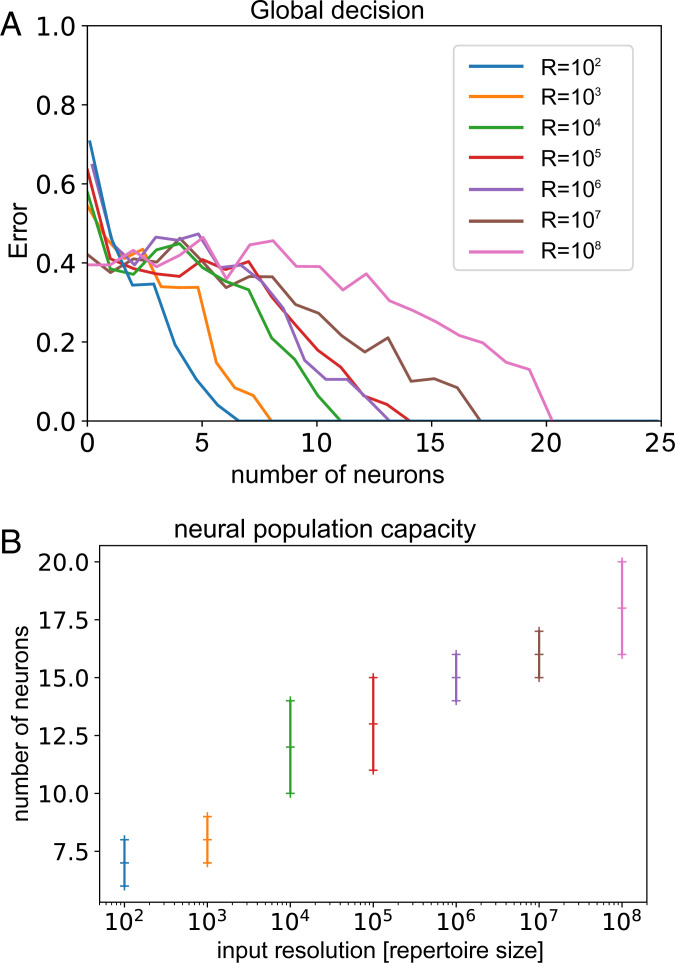
We propose that coding and decoding in the brain are achieved through digital computation using three principles: relative ordinal coding of inputs, random connections between neurons, and belief voting. Due to randomization and despite the coarseness of the relative codes, we show that these principles are sufficient for coding and decoding sequences with error-free reconstruction. In particular, the number of neurons needed grows linearly with the size of the input repertoire growing exponentially. We illustrate our model by reconstructing sequences with repertoires on the order of a billion items. From this, we derive the Shannon equations for the capacity limit to learn and transfer information in the neural population, which is then generalized to any type of neural network. Following the maximum entropy principle of efficient coding, we show that random connections serve to decorrelate redundant information in incoming signals, creating more compact codes for neurons and therefore, conveying a larger amount of information. Henceforth, despite the unreliability of the relative codes, few neurons become necessary to discriminate the original signal without error. Finally, we discuss the significance of this digital computation model regarding neurobiological findings in the brain and more generally with artificial intelligence algorithms, with a view toward a neural information theory and the design of digital neural networks.

Keywords: catastrophic forgetting; continual learning; digital computing; maximum entropy; sparse coding.

Fig. 1.

Schematic presentation of the neural population based on randomly permuted ordinal codes. The process has three stages: the encoding of the original sequence, its decoding, and a global belief vote. In the first phase, the neurons encode the relative order (the ranks) of the items in the spatiotemporal sequence X using multiple randomly shuffled orderings of the item alphabet. The result is that each neuron sees a randomly permuted ordinal code [e.g., $P(Y/X)$]. The items’ values are no longer present in the ordinal codes, which perform a drastic quantization of information. During the decoding phase, each neuron reconstructs the sequence in its alphabet ordering by trial and error [e.g., $Q(X/Y)$]. Thus, each neuron has a different local estimate of the items in the sequence. In the final stage, after mapping back the local alphabet orderings to the original, a global belief vote at the population level accumulates the local decisions from all the neurons, allowing correction of local decision errors (e.g., maximum a posteriori probability $\widehat{X}=X^{*}$).

Fig. 2.

Robust neural decoding of a signal encoded with and without random permutation of the input repertoire (alphabet). (A) Encoding using N neurons without permuting the alphabet order. Local (per neuron) errors are modeled by a Gaussian distribution. Combining the N local estimates (top) allows only for a linear reduction in the estimation noise through averaging. (B) Random alphabet permutations cause repertoire items that are neighbors in the original order to lie farther apart. When cumulating the reordered local Gaussian votes (top), this leads to a nonlinear effect that lets the global estimate stand out in the noise, which is now spread over the entire alphabet.

Fig. 3.

Efficiency of a relative order code vs. a temporal code. (A) A spatiotemporal sequence of L items taken in a repertoire of size R. (B) Ordinal codes represent the sequence with a vector from L only, storing the relative rank order over time of the items in the sequence. In C and D, in terms of computational cost and precision, formal neurons, such as perceptrons, have to encode the items’ index of temporal sequences in their synaptic weights either with resolution R and L synaptic links or with R synaptic links and synaptic weights with resolution L. In C, instead, ordinal codes represent in their weights the relative order of items in the sequence only (L values). In D, this second type of coding allows for the drastic quantization of information to only L synaptic links to learn, with respect to the R links necessary instead, as in formal neurons. This large reduction in dimensionality comes at the cost of losing information about the items’ values.

Fig. 4.

Examples of reconstructed sequences with different permuted alphabets or keys, with R = 100 and L = 50. The permuted ordinal code learned by each neuron allows us to retrieve the sequence with high fidelity but always with some small local error due to the quantization to ranks performed by the neurons in their respective alphabet order (A–D). The original sequence (in the permuted order alphabet A_i of the neuron i) is plotted in blue, and the retrieved sequence is plotted in red. Variance is proportional to R, approximately $\pm 0.1R$.

Fig. 5.

Local decision vote for individual neurons and global decision vote at the neural population level: R = 100, L = 50. The red arrow indicates the true value to be retrieved back. In A, the activity level represents the local decision vote for each neuron (x axis) based on the Gaussian density distribution centered on the estimated values for each item in their respective randomized alphabet (y axis). B presents the cumulative sum with respect to the number of neurons used during global decision. The activity level indicates the accumulated sum for each item: the global decision vote at the neural population level. C displays the cumulative sum for several numbers of neurons used.

Fig. 6.

Plot of the RMSE for the global decision at the neural population level with respect to the parameter $\sigma \in [1,5,10,20,50]$, with R = 100 and L = 50. The smaller the parameter σ is, the less effective the decision-making, which will not make good use of the redundancy. In such cases, 10 neurons are not enough to retrieve the original sequence, limited to an RMSE of 0.3. Instead, for a larger parameter σ above 10, fewer neurons can drastically reduce error to zero, performing a sparse coding of the incoming sequence.

Fig. 7.

Sequence reconstruction vs. the number of neurons N for a fixed input sequence of length $L=50$ (repertoire size $R={10}^7$). Each column in the matrix plot corresponds to the reconstruction for a given N. A shows the global reconstruction in the color-coded repertoire. (B) The squared reconstruction error averaged over the neurons. Approximately 17 neurons are needed to guarantee correct reconstruction in all sequence positions.

Fig. 8.

The number of neurons needed to decode a sequence of various resolutions. The resolution is related to the size R of the input repertoire or its cardinality, from which items are taken in the sequence (larger R for finer resolution). The number of neurons N_limit is the minimum number of neurons found necessary for reconstruction without error. (A) The global decision vote for various cardinalities R. We set σ to the large value $R/2$. In B, the minimum number of neurons needed is N_limit to reconstruct the sequence without error with respect to the input resolution (R, respectively). The graph shows a linear progression of the number of neurons required to code a sequence while the cardinality R augments exponentially; the values are averaged over 10 simulations.

Fig. 9.

Image reconstruction by neurons of lower resolution. In A, we present two neurons that encode an image with random permutations of the pixels’ distribution (255 values) and reduced to a binary code (two values). (C) Euclidean error with respect to the number of neurons used during global decision-making. Nearly 40 binary neurons are required to retrieve back perfectly the original pixels’ value. (D) Image reconstruction for different numbers of neurons used during the decision vote.

References

1. Barlow H., “Possible principles underlying the transformation of sensory messages” in Sensory Communication, Rosenblith W., Ed. (MIT Press, Cambridge, MA, 1961), pp. 217–234.
1. Baddeley R., Hancock P. J., Földiák P., Information Theory and the Brain (Cambridge University Press, Cambridge, United Kingdom, 2000).
1. Laughlin S. B., Sejnowski T. J., Communication in neuronal networks. Science 301, 1870–1874 (2003). - PMC - PubMed
1. Olshausen B. A., Field D. J., Sparse coding of sensory inputs. Curr. Opin. Neurobiol. 14, 481–487 (2004). - PubMed
1. Rolls E. T., Treves A., The neuronal encoding of information in the brain. Prog. Neurobiol. 95, 448–490 (2011). - PubMed
Publication types
LinkOut - more resources