Bayesian emulation and history matching of JUNE
- PMID: 35965471
- PMCID: PMC9376712
- DOI: 10.1098/rsta.2022.0039
Bayesian emulation and history matching of JUNE
Abstract
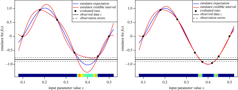
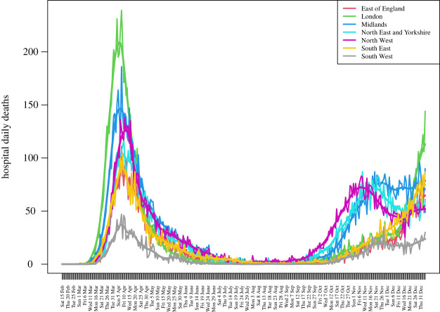
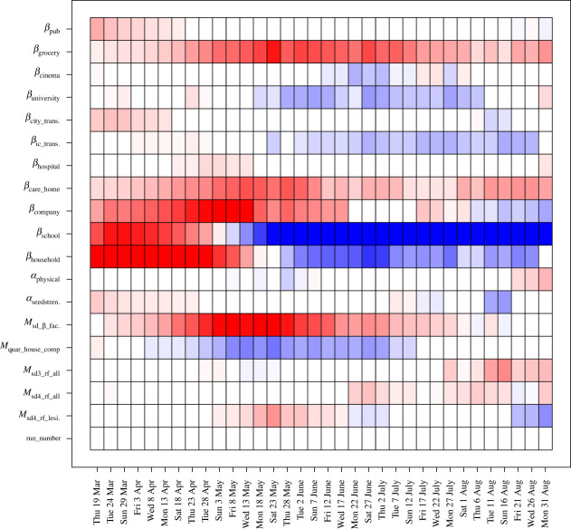
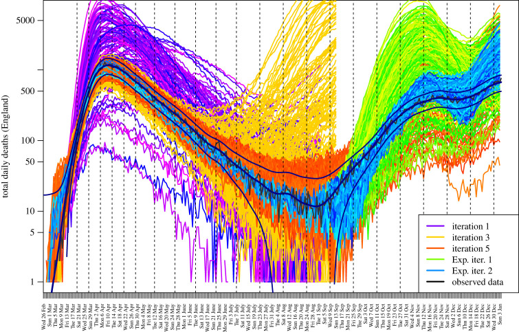
We analyze JUNE: a detailed model of COVID-19 transmission with high spatial and demographic resolution, developed as part of the RAMP initiative. JUNE requires substantial computational resources to evaluate, making model calibration and general uncertainty analysis extremely challenging. We describe and employ the uncertainty quantification approaches of Bayes linear emulation and history matching to mimic JUNE and to perform a global parameter search, hence identifying regions of parameter space that produce acceptable matches to observed data, and demonstrating the capability of such methods. This article is part of the theme issue 'Technical challenges of modelling real-life epidemics and examples of overcoming these'.
Keywords: Bayes linear; calibration; disease models; emulation; history matching.
Figures
Similar articles
-
Technical challenges of modelling real-life epidemics and examples of overcoming these.Philos Trans A Math Phys Eng Sci. 2022 Oct 3;380(2233):20220179. doi: 10.1098/rsta.2022.0179. Epub 2022 Aug 15. Philos Trans A Math Phys Eng Sci. 2022. PMID: 35965472 Free PMC article.
-
Bayesian uncertainty analysis for complex systems biology models: emulation, global parameter searches and evaluation of gene functions.BMC Syst Biol. 2018 Jan 2;12(1):1. doi: 10.1186/s12918-017-0484-3. BMC Syst Biol. 2018. PMID: 29291750 Free PMC article.
-
Estimation of local time-varying reproduction numbers in noisy surveillance data.Philos Trans A Math Phys Eng Sci. 2022 Oct 3;380(2233):20210303. doi: 10.1098/rsta.2021.0303. Epub 2022 Aug 15. Philos Trans A Math Phys Eng Sci. 2022. PMID: 35965456 Free PMC article.
-
The importance of uncertainty quantification in model reproducibility.Philos Trans A Math Phys Eng Sci. 2021 May 17;379(2197):20200071. doi: 10.1098/rsta.2020.0071. Epub 2021 Mar 29. Philos Trans A Math Phys Eng Sci. 2021. PMID: 33775141 Free PMC article.
-
Parameter estimation and uncertainty quantification using information geometry.J R Soc Interface. 2022 Apr;19(189):20210940. doi: 10.1098/rsif.2021.0940. Epub 2022 Apr 27. J R Soc Interface. 2022. PMID: 35472269 Free PMC article. Review.
Cited by
-
Estimation of age-stratified contact rates during the COVID-19 pandemic using a novel inference algorithm.Philos Trans A Math Phys Eng Sci. 2022 Oct 3;380(2233):20210298. doi: 10.1098/rsta.2021.0298. Epub 2022 Aug 15. Philos Trans A Math Phys Eng Sci. 2022. PMID: 35965466 Free PMC article.
-
Technical challenges of modelling real-life epidemics and examples of overcoming these.Philos Trans A Math Phys Eng Sci. 2022 Oct 3;380(2233):20220179. doi: 10.1098/rsta.2022.0179. Epub 2022 Aug 15. Philos Trans A Math Phys Eng Sci. 2022. PMID: 35965472 Free PMC article.
-
Emulating computer models with high-dimensional count output.Philos Trans A Math Phys Eng Sci. 2025 Mar 13;383(2292):20240216. doi: 10.1098/rsta.2024.0216. Epub 2025 Mar 13. Philos Trans A Math Phys Eng Sci. 2025. PMID: 40078142 Free PMC article.
-
Challenges and opportunities in uncertainty quantification for healthcare and biological systems.Philos Trans A Math Phys Eng Sci. 2025 Mar 13;383(2292):20240232. doi: 10.1098/rsta.2024.0232. Epub 2025 Mar 13. Philos Trans A Math Phys Eng Sci. 2025. PMID: 40078151 Free PMC article. Review.
-
Visualization for epidemiological modelling: challenges, solutions, reflections and recommendations.Philos Trans A Math Phys Eng Sci. 2022 Oct 3;380(2233):20210299. doi: 10.1098/rsta.2021.0299. Epub 2022 Aug 15. Philos Trans A Math Phys Eng Sci. 2022. PMID: 35965467 Free PMC article.
References
-
- Vernon I, Goldstein M, Bower RG. 2010. Galaxy formation: a Bayesian uncertainty analysis. Bayesian Anal. 5, 619-670. (10.1214/10-ba524) - DOI
-
- Williamson D, Goldstein M, Allison L, Blaker A, Challenor P, Jackson L, Yamazaki K. 2013. History matching for exploring and reducing climate model parameter space using observations and a large perturbed physics ensemble. Clim. Dyn. 41, 1703-1729. (10.1007/s00382-013-1896-4) - DOI
-
- Craig PS, Goldstein M, Seheult AH, Smith JA. 1997. Pressure matching for hydrocarbon reservoirs: a case study in the use of Bayes linear strategies for large computer experiments (with discussion). In Case Studies in Bayesian Statistics (eds C Gatsonis, JS Hodges, RE Kass, R McCulloch, P Rossi, ND Singpurwalla), vol. 3, pp. 36–93. New York: Springer-Verlag.
MeSH terms
Grants and funding
LinkOut - more resources
Full Text Sources
Medical