The origin and evolution of open habitats in North America inferred by Bayesian deep learning models

Abstract

Some of the most extensive terrestrial biomes today consist of open vegetation, including temperate grasslands and tropical savannas. These biomes originated relatively recently in Earth's history, likely replacing forested habitats in the second half of the Cenozoic. However, the timing of their origination and expansion remains disputed. Here, we present a Bayesian deep learning model that utilizes information from fossil evidence, geologic models, and paleoclimatic proxies to reconstruct paleovegetation, placing the emergence of open habitats in North America at around 23 million years ago. By the time of the onset of the Quaternary glacial cycles, open habitats were covering more than 30% of North America and were expanding at peak rates, to eventually become the most prominent natural vegetation type today. Our entirely data-driven approach demonstrates how deep learning can harness unexplored signals from complex data sets to provide insights into the evolution of Earth's biomes in time and space.

Fig. 1. The process of feature generation.

The workflow is shown exemplarily for one point with current vegetation information (framed in red), located at the coordinates −125, 60 (Decimal Degree System) and labeled as “closed” vegetation. Our database, compiled for this study, contains other points with current or past vegetation information, labeled as open (grass symbol) or closed (tree symbol). Once the model is trained it can be applied to estimate the vegetation interpretation for points in space and time, which are currently lacking such information (represented by the question mark). For the selected point, defined by its longitude (Lon), latitude (Lat), and age, we extract several abiotic features, reflecting climatic, geographic, and temporal variables (see box “Abiotic features”). In addition, we extract the spatial distance to the closest occurrence of each taxon in our occurrence database (see box “Biotic distances”). This is repeated for each geological stage (n = 17), while also extracting the temporal distance between the given point and the mid age of each geological stage. In the example the temporal distance to the nearest horse occurrence in stage 1 is 0 (see cells highlighted in red) because the vegetation point falls within this first geological stage.

Fig. 2. The BNN model architecture.

a The spatial and temporal distances extracted separately for 100 mammal and plant taxa (Fig. 1), are the input of the first two hidden layers in the BNN model. During training, the BNN optimizes weights (represented by lines labeled with $w_X$) to reduce the multitude of spatial and temporal distance measurements into one single “proximity” value for each taxon (taxon nodes) relative to the given point in space and time. This process of feature generation is equivalent to the convolutional layers in an image classifier, reducing higher-dimensionality data into lower-dimensionality features for input into the subsequent neural network layers. In some of our tested models the resulting taxon features are pooled before being passed on to the next layer. b The taxon node values (“Biotic features”) are then used in combination with the abiotic features as input into the fully connected BNN classifier layers. Jointly with the weights of the feature generation layers, the weights of the BNN classifier are estimated during training through MCMC sampling, to optimally map the input data to the correct output vegetation label (“open” or “closed”). Once trained, a posterior sample of the weights is stored for each model and is used to make vegetation predictions for points with unknown vegetation interpretation.

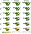
Fig. 3. Vegetation predictions for North America throughout the last 25 Myr.

The predictions are based on the best model resulting from our model evaluation and sensitivity tests (model 1, Table 1). Column a shows the posterior probability (PP) estimates for open habitat, where a PP of >0.95 (yellow) indicates strong evidence for open habitat, whereas a PP of <0.05 (green) indicates strong evidence for closed habitat. Columns b and c show categorical vegetation class predictions for our vegetation classes “open” (yellow) and “closed” (green). The class predictions are based on a PP threshold ensuring 90% prediction accuracy (b), and 95% prediction accuracy (c), respectively. The higher the applied PP threshold, the more sites will be classified as “unknown” (gray). Source data are provided as a Source data file.

Fig. 4. Predicted fraction of open vegetation through time.

Fractions are calculated as the proportion of all terrestrial cells across North America predicted as open vegetation with the best model (model 1). The solid yellow line shows the mean estimates across all posterior samples, while the shaded area shows the 95% highest posterior density (HPD) interval. The blue line shows the mean rate of open habitat expansion, calculated across each preceding 1-million-year time bin. The colored bar forming the x-axis marks the geological epochs covered by our predictions, including the Pleistocene (PE), Pliocene (PL), Miocene, and Oligocene (not shown is the Holocene, from 0.01 Ma to present). The small panels show histograms of the posterior estimates of open vegetation fraction (95% HPD), marking important points in time for open vegetation evolution. These points highlight (i) 23 Ma, the earliest time where our model predicts the presence of open vegetations with confidence (>95% HPD); (ii) 5 Ma, beginning of Pliocene and the start of an acceleration in open vegetation expansion; and (iii) 2–3 Ma, beginning of Pleistocene epoch, marking the highest rate of open vegetation expansion. Source data are provided as a Source data file.

Fig. 5. Impact of individual features on model prediction accuracy.

The displayed delta-accuracy values (y-axis) constitute a measure of how important a given feature is for the trained model to make accurate vegetation predictions. This is determined by measuring the drop in prediction accuracy when the information content of a given feature is removed (permutation feature importance). High delta accuracy values indicate high feature importance. Points show the mean delta-accuracy of each feature across 100 randomly selected posterior BNN weight samples. The inserted panel (“All features”) displays an overview of the delta-accuracy estimates for all 108 features, while the main panel displays only the most important features for the trained model. Note that the feature importance determined in this way is not an absolute measure of how important a given predictor is for the task of vegetation prediction, but rather it is an assessment of how much a given model relies on a given predictor. The identity of the most important features may change depending on the model architectures, even when based on the same data. However, the most important features identified in this manner are expected to contain relevant information for the given task, in this case for reconstructing vegetation. Source data are provided as a Source data file.

References

1. Lu Z, et al. Vegetation pattern and terrestrial carbon variation in past warm and cold climates. Geophys. Res. Lett. 2019;46:8133–8143. doi: 10.1029/2019GL083729. - DOI
1. Peppe DJ. Megafloral change in the early and middle Paleocene in the Williston Basin, North Dakota, USA. Palaeogeogr., Palaeoclimatol., Palaeoecol. 2010;298:224–234. doi: 10.1016/j.palaeo.2010.09.027. - DOI
1. Janis CM. A climatic explanation for patterns of evolutionary diversity in ungulate mammals. Palaeontology. 1989;32:463–481.
1. Carvalho MR, et al. Extinction at the end-Cretaceous and the origin of modern Neotropical rainforests. Science. 2021;372:63–68. doi: 10.1126/science.abf1969. - DOI - PubMed
1. Niklas KJ, Tiffney BH, Knoll AH. Patterns in vascular land plant diversification. Nature. 1983;303:614–616. doi: 10.1038/303614a0. - DOI
Publication types