Natural switches in behaviour rapidly modulate hippocampal coding

Abstract

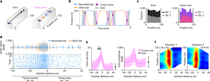
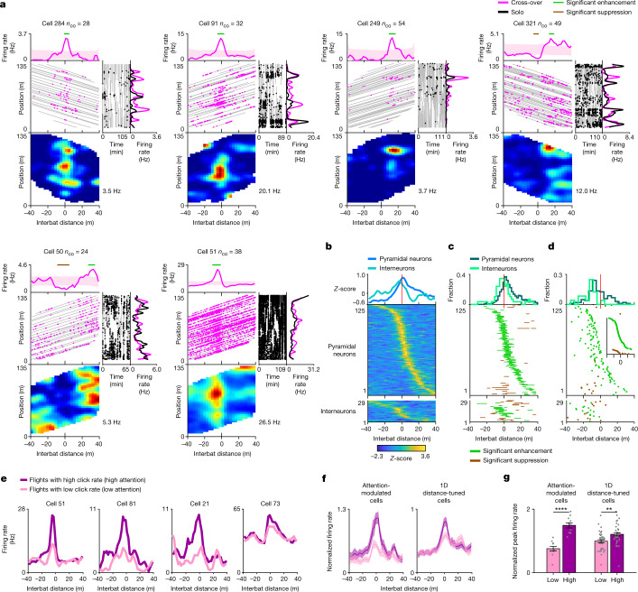
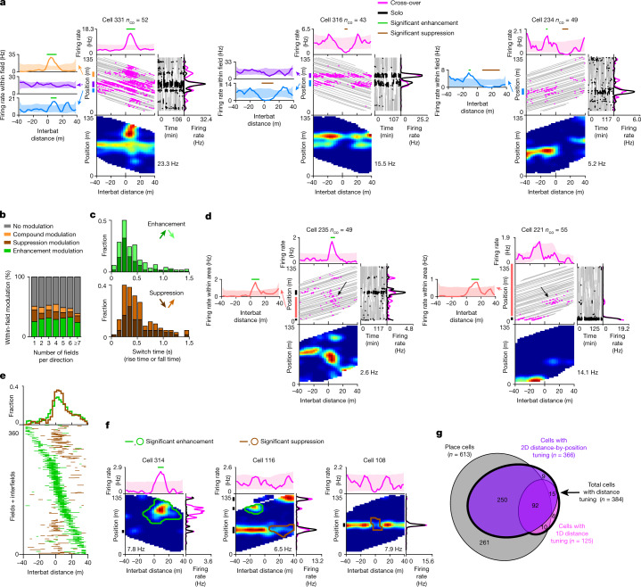
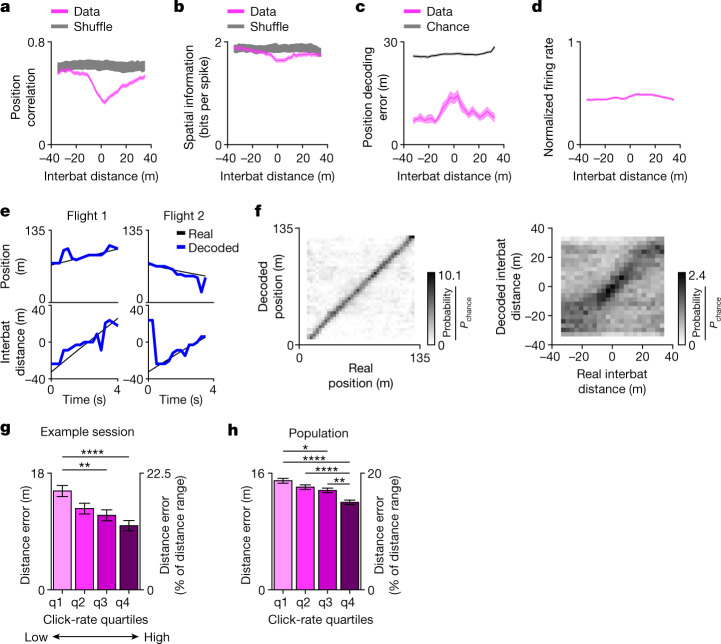
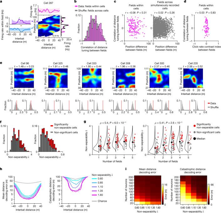
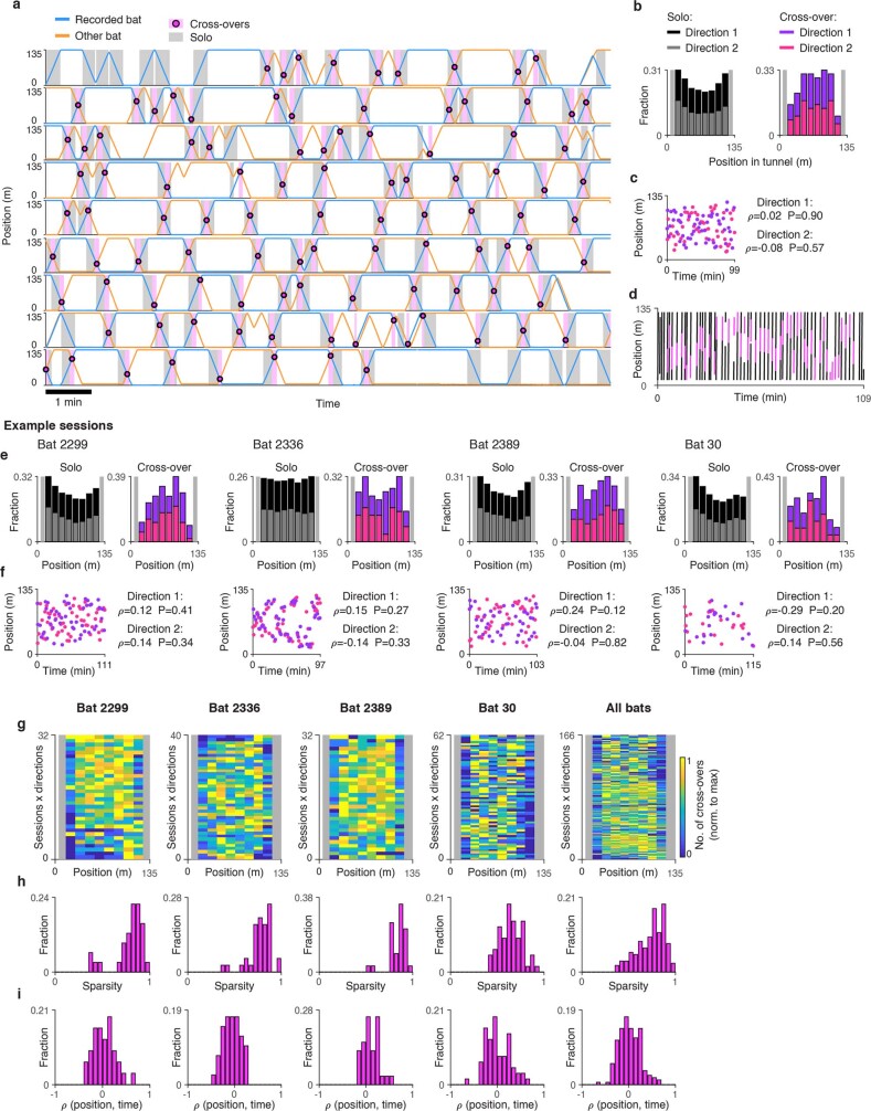
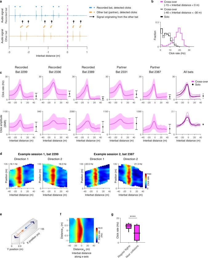
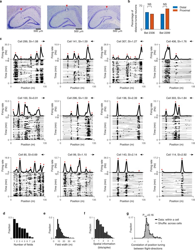
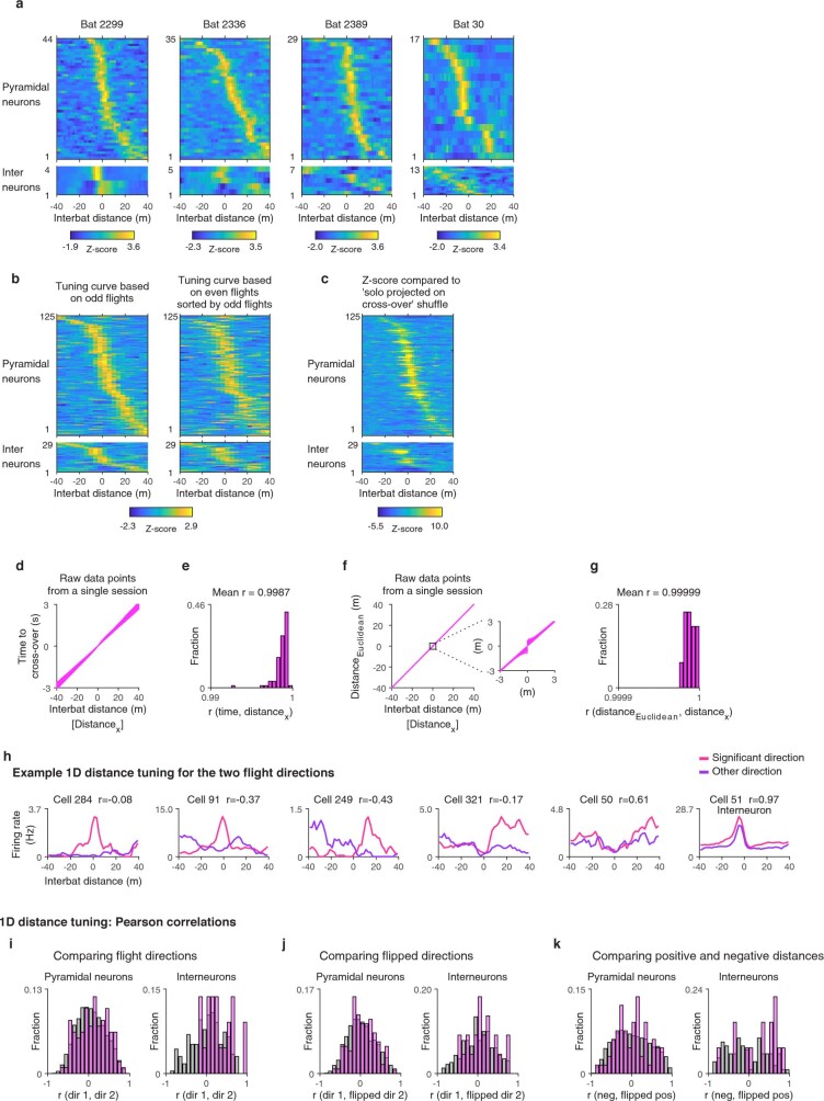
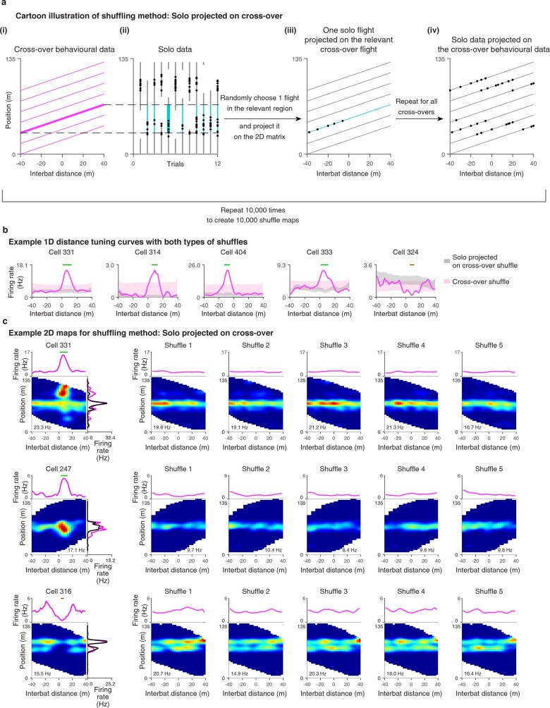
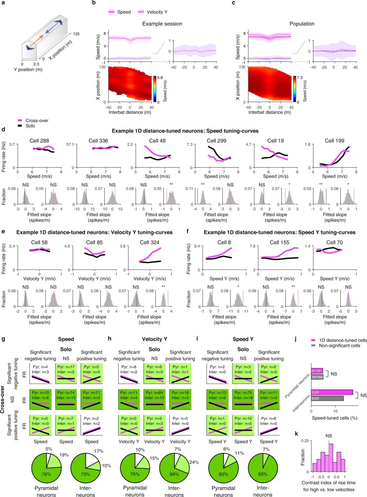
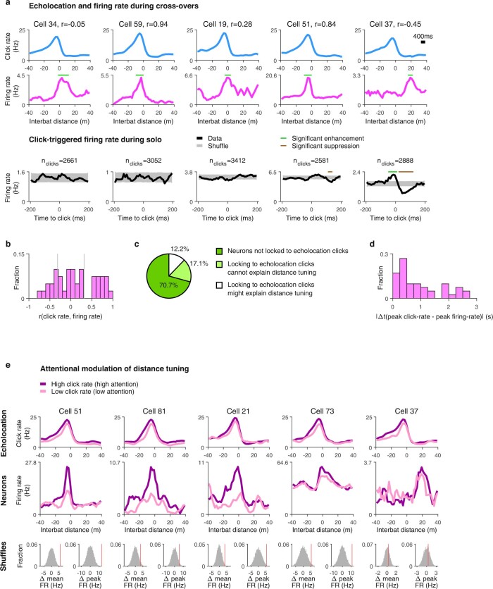
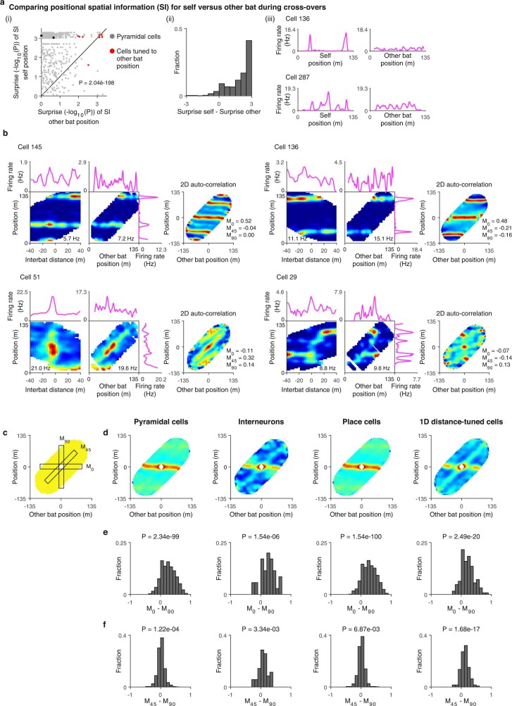
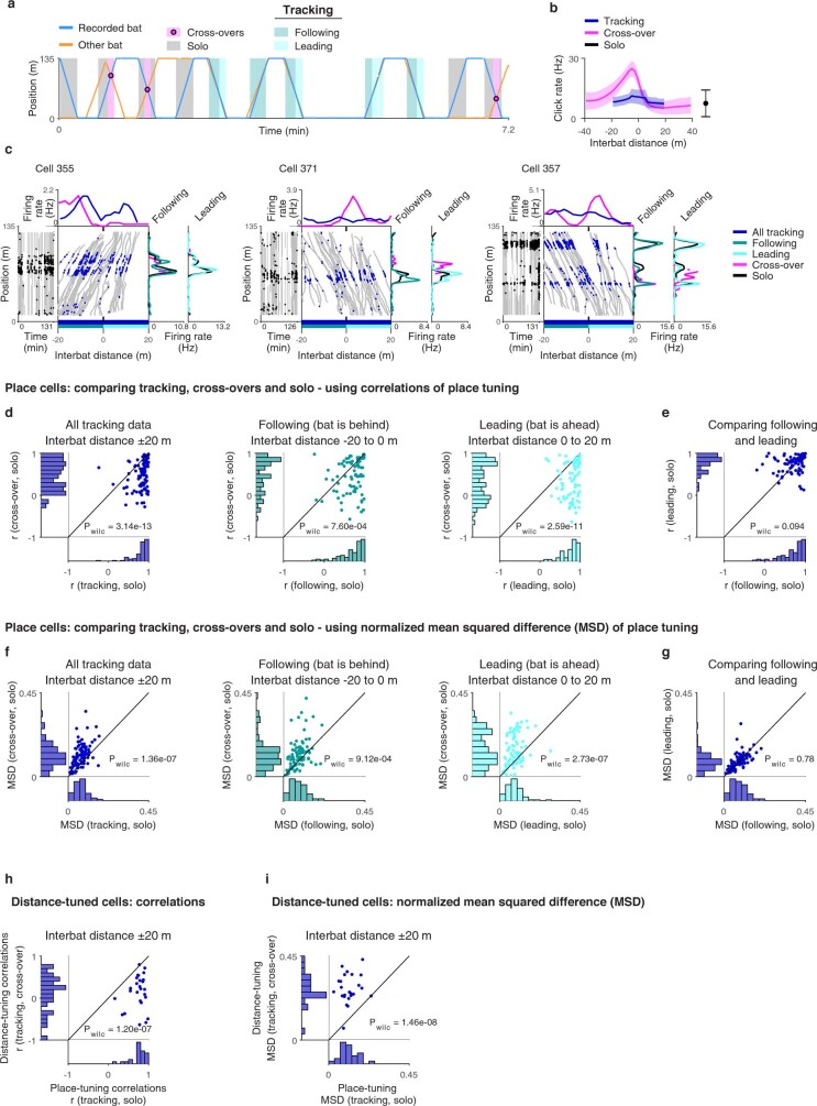
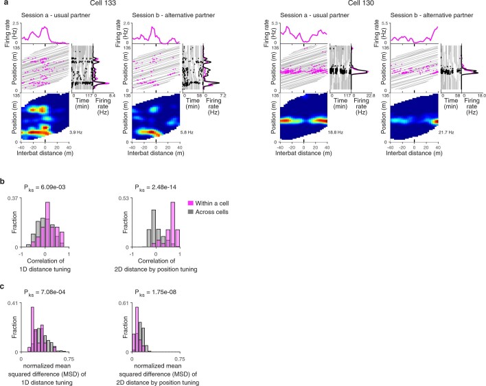
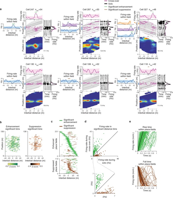
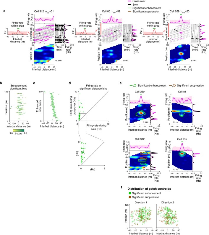
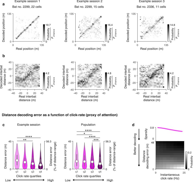
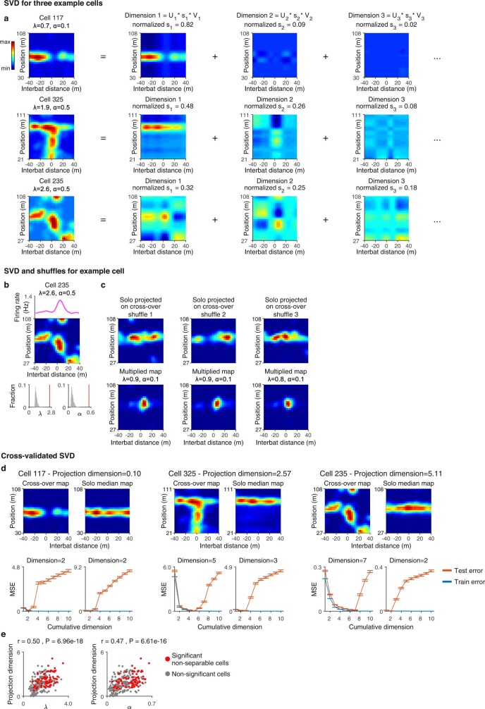
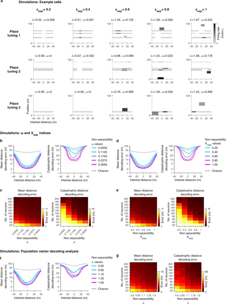
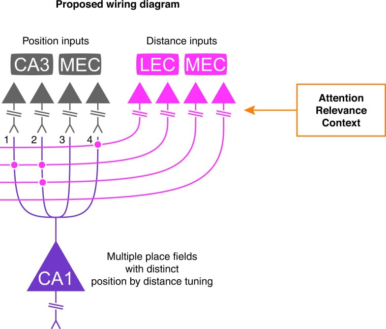
Throughout their daily lives, animals and humans often switch between different behaviours. However, neuroscience research typically studies the brain while the animal is performing one behavioural task at a time, and little is known about how brain circuits represent switches between different behaviours. Here we tested this question using an ethological setting: two bats flew together in a long 135 m tunnel, and switched between navigation when flying alone (solo) and collision avoidance as they flew past each other (cross-over). Bats increased their echolocation click rate before each cross-over, indicating attention to the other bat^1-9. Hippocampal CA1 neurons represented the bat's own position when flying alone (place coding^10-14). Notably, during cross-overs, neurons switched rapidly to jointly represent the interbat distance by self-position. This neuronal switch was very fast-as fast as 100 ms-which could be revealed owing to the very rapid natural behavioural switch. The neuronal switch correlated with the attention signal, as indexed by echolocation. Interestingly, the different place fields of the same neuron often exhibited very different tuning to interbat distance, creating a complex non-separable coding of position by distance. Theoretical analysis showed that this complex representation yields more efficient coding. Overall, our results suggest that during dynamic natural behaviour, hippocampal neurons can rapidly switch their core computation to represent the relevant behavioural variables, supporting behavioural flexibility.

Fig. 1. Set-up and behavioural task.

a, The experimental set-up. Bats flew in pairs and alternated between two behavioural modes: solo (left) and cross-over (right). b, Example behaviour (4 min of the full session that is shown in Extended Data Fig. 1a). The blue and orange lines show the positions of the recorded bat and the other bat, respectively; the pink circles show cross-over events; pink rectangles show cross-over flights (±40 m distance around cross-over events); grey rectangles show solo flights. c, The distribution of behavioural coverage along the tunnel in an example session: solo (left) and cross-over (right) flight is shown separately for the two flight directions (dir.) (dark and light coloured, stacked). The light grey vertical rectangles show the areas in which cross-overs were not analysed (Methods). d, Echolocation example. Top, the audio signal during one cross-over flight for the recorded bat (blue) and for the other bat (orange) as a function of the interbat distance (negative/positive distances: bats flying towards/away from each other). Bottom, raster plot showing the echolocation clicks of the recorded bat (blue dots) for the 50 cross-overs in this session (one flight direction). Note that Egyptian fruit bats emit pairs of clicks. SNR, signal-to-noise ratio. e, The population average echolocation click rate (left) and click amplitude (right) for bat 2299 (n = 11 sessions) during cross-over flight (data are mean ± s.d. (pink shading), with the s.d. computed over all behavioural data in each distance bin) and solo flight (data are mean ± s.d.). Scale bar, the mean distance flown in 1 s. f, 2D click rate maps for interbat distance (x axis) by position (y axis) for the two flight directions for all sessions of bat 2299, coloured from zero (blue) to peak click rate (red; value indicated). Note that the click rate increased before cross-over, similarly along all of the positions (see the vertical band). Source data

Fig. 2. Hippocampal CA1 neurons represent the distance to another bat upon brief attentional switches during navigation.

a, Examples of 1D distance neurons. n_co represents the number of cross-overs. For each cell, the top row shows the tuning curve for 1D distance (pink line) and shuffles (shading). Horizontal lines denote significant enhancement (green) or suppression (brown). In the middle row, the left plot shows the recorded bat position (y axis) and interbat distance (x axis) during cross-overs (grey; the two flight directions yield positive versus negative slopes of the grey lines), with spikes overlaid (pink dots); the centre plot shows the spike raster during solo flights (grey, behaviour; black dots, spikes), showing position (y axis) versus time in the session (x axis; the solo raster has holes in which cross-overs occurred; Extended Data Figs. 1d and 3c); and the right plot shows place tuning during solo flights (black) and during cross-over flights (pink). The bottom row shows the 2D firing-rate map of position (y axis) by interbat distance (x axis), coloured from zero (blue) to peak firing rate (red; value indicated). b–d, Population summary of all significant 1D distance neurons for putative pyramidal neurons (n = 125) and interneurons (n = 29). b, Top, the mean of z-scored distance tuning curves. A raster of z-scored tuning curves is shown separately for pyramidal neurons (middle) and interneurons (bottom), sorted by peak distance. c, Top, the fraction of cells with significant distance enhancement, as a function of interbat distance. Significantly enhanced and suppressed bins for pyramidal neurons (middle) and interneurons (bottom) are shown. d, Top, the distribution of enhancement response onset (the distance at which the tuning crossed 90% of the shuffle distribution). The response onset for pyramidal neurons (middle) and interneurons (bottom) is shown. Inset, pyramidal cells sorted by onset distance (separately for enhancement and suppression). e–g, Attentional modulation of distance tuning, comparing higher-click-rate flights (purple, high attention) with lower-click-rate flights (pink, low attention). e, Example cells: 1D distance tuning curves. f, The average population tuning curves (each cell was normalized to its peak firing rate computed using all flights) for all 1D distance neurons (right) and all cells significantly modulated by click rate (left). g, The peak firing rate (normalized as described in f), for high- and low-click-rate flights (purple and pink), plotted for 1D distance neurons (right; one-tailed t-test: t = 2.47, P = 0.009, n = 37 cells × directions), and neurons that were significantly modulated by click rate (left; one-tailed t-test: t = 6.44, P = 3.72 × 10⁻⁵, n = 11). For f and g, data are mean ± s.e.m. Source data

Fig. 3. Conjunctive representation of interbat distance by position.

a, Examples of three neurons. For each cell, the middle and right plots are as described in Fig. 2a, and the left plot shows the 1D distance tuning curves within different place fields (colours correspond to different place fields, marked by vertical coloured lines on the left of the centre plot). Place fields here and elsewhere were defined on the basis of solo data. Shading shows cross-over shuffles; horizontal green and brown lines show bins with significant enhancement and suppression, respectively. b, The percentages of different types of distance modulation within place fields for neurons with different numbers of place fields. Compound modulation indicates tuning with both significant enhancement and suppression (for example, cell 234 (blue) in a). c, The distribution of neuronal switch times of the distance tuning. Top, the rise time (dark green) and fall time (light green; stacked) for place fields with significantly enhanced distance tuning curves. n = 143. Bottom, the fall time (dark brown) and rise time (light brown) for place fields with significantly suppressed distance tuning curves. n = 62. Only a subset of the fields was valid for analysis here (Methods). d, Examples of two neurons with significant enhancement outside their place fields (within an interfield), plotted as described in a. The vertical lines on the left of the centre panel mark place fields (black) and interfields (peach). The black arrows indicate spikes contributing to distance tuning within the interfield; note that there were barely any spikes in the same position during solo flights (see the solo raster on the right). e, Population summary: distance bins that were significantly enhanced (green) or suppressed (brown) within place fields (n = 301 fields) and interfields (n = 59) sorted by distance-tuning peak. f, 2D distance by position tuning: patch analysis. Examples of cells with significant 2D patches are plotted as described in Fig. 2a without the raw data panels. The outlines show significant 2D patches (enhancement (green); suppression (brown)). The vertical black lines show place fields. g, Summary of different functional classes of pyramidal cells (numbers denote cells × directions). Place cells are shown in grey. The thick black curve encompasses the total number of distance-modulated cells (n = 384, 55.4% of all pyramidal cells). Source data

Fig. 4. Simultaneous decoding of interbat distance and position.

a–d, Change of position tuning during cross-overs. a, The average Pearson correlation between position tuning during solo and during cross-over flights, computed in 10-m distance bins (Methods). Data are mean ± s.e.m. (pink). n = 613 place cells × directions. Note the correlations decreased when bats approached each other, indicating a change in position tuning. The grey curve was computed as described for the pink curve, using solo projected on cross-over shuffles. b, Spatial information (mean ± s.e.m.; n = 613 place cells × directions) for the position-tuning curves computed during cross-over flights (pink), and for solo projected on cross-over shuffles (grey). c, Position decoding error as a function of distance during cross-over (pink; mean ± s.e.m.; n = 16 sessions) and chance level (grey). Note the increased decoding error at short distances. d, Firing rate (normalized to the peak of each cell) as a function of distance during cross-over for all place cells. Data are mean ± s.e.m. n = 613 place cells × directions. e,f, Simultaneous decoding of the interbat distance and position during cross-over flights. e, Examples of two flights (columns). Top, real position (black) and decoded position (blue) versus time. Bottom, real and decoded interbat distance. f, Confusion matrices (pooled over all sessions with ≥10 cells recorded simultaneously; n = 16 sessions). Left, the probability of decoded positions (y axis) for each real position (x axis), normalized to the uniform chance probability P_chance = 1/n_bins (colour bar). Right, the same for the interbat distance. The diagonal structure in these matrices indicates accurate and unbiased decoding. g,h, The decoding error of interbat distance for different click-rate quartiles (q1–q4, quartiles of low click rate to high click rate) for one example session (g) (n = 146, n = 134, n = 146 and n = 151 decoding time windows for q1–q4) or pooled over all nine sessions that had audio recordings and ≥10 cells (h) (n = 998, n = 1,051, n = 1,074 and n = 1,063 decoding time windows for q1–q4). Note that the decoding error decreased as the click rate increased (q4, maximal click rate, that is, maximal attention; click rate is a proxy of attention). Data are mean ± s.e.m. Statistical analysis was performed using analysis of variance with post hoc correction for multiple comparisons: *P < 0.05, **P < 0.01, ***P < 0.001, ****P < 0.0001; no asterisks, not significant. See Extended Data Fig. 13c for the exact P values, violin plots and Kruskal–Wallis tests. Source data

Fig. 5. The representation of distance by position is complex and non-separable.

a–d, Different distance tuning across different place fields. a, Example cell. Note the two place fields showed opposite distance modulation. b, The distribution of Pearson correlations between the 1D distance tuning curves of pairs of place fields of the same cell (pink; n = 170 pairs; the inclusion criteria are described in the Methods), or place fields of different simultaneously recorded cells (grey, cell shuffling; n = 2,479 pairs). c, Pearson correlations between the 1D distance tuning curves of pairs of place fields of the same cell (left) or of simultaneously recorded different cells (right), plotted versus the position difference between the place-field peaks (Pearson correlations of the scatters are indicated). d, Pearson correlations between the 1D distance tuning curves of pairs of place fields of the same cell (y axis) and the contrast index of echolocation click rate during cross-over within these pairs of place fields (x axis; contrast index = (CR_field1 − CR_field2) / (CR_field1 + CR_field2), where CR is the click rate). n = 79 pairs of place fields recorded with audio. e–g, SVD analysis shows non-separable distance-by-position coding. e, Example neurons with varying degrees of non-separability. Top, 2D firing rate map of position (y axis) by interbat distance (x axis), cropped and completed for the SVD analysis (Methods); λ and α (non-separability indices) are indicated: higher values denote non-separable cells; neurons are sorted by λ. Bottom, histograms of shuffle distributions (grey) and real values (red lines) for λ (left) and α (right). Cell 96 is separable (two place fields show same distance tuning), the other five cells are significantly non-separable (different distance modulations at different positions). f, The distributions of λ and α across all cells in the SVD analysis (n = 262 cells × directions; inclusion criteria are described in the Methods). Grey, non-significant cells (n = 189 cells × directions). Red, significantly non-separable cells (n = 73 cells × directions). g, Non-separability indices λ and α versus the number of place fields of the cell (only place fields within the SVD rectangular maps were included; n = 237 place cells × directions). Spearman correlation ρ values are indicated. The black dots show the median; and the black lines are kernel density plots. h,i, The functional advantage of non-separability: theoretical analysis of distance decoding for simulated neurons. h, Mean decoding error (left) and catastrophic decoding error (right, 99th percentile of errors), plotted on a log scale as a function of the interbat distance, separately for simulated populations of cells with different non-separability values, λ (different colours). Grey, chance-level decoding. i, Mean decoding error (left, colour-coded) and catastrophic decoding error (right) as a function of the number of neurons used for decoding and the non-separability index, λ. Source data

Extended Data Fig. 1. Solo and cross-over behaviours were intermingled and distributed quite uniformly along the tunnel.

a–d, Example of one experimental session: same experimental session as shown in Fig. 1b. a, The positions of the two bats along the entire experimental session. Time in session runs from top-left to bottom-right; scale bar, 1 min. Blue and orange lines: positions of the recorded bat and other bat, respectively. Cross-over events are marked with pink circles, and cross-over flights (window of ±40-m of interbat distance around the cross-over event) are marked with pink rectangles. Solo flights are marked with grey rectangles. b, Distribution of behavioural coverage along the tunnel: Solo (left) and cross-overs (right), plotted separately for the two flight-directions (dark and light-coloured, stacked). Light grey vertical rectangles at the edges of both panels: areas where cross-overs were not analysed (Methods); we also note that there were less cross-overs in the bins adjacent to the grey rectangles (see also panels e and g). c, Position versus time within the session (time from first to last cross-over), for all the cross-over events in the session shown in a. The cross-over events occurred quite uniformly along the entire tunnel (y axis), and were pseudo-randomly distributed over time (x axis; direction 1, Spearman correlation of position versus time: ρ = 0.02, P = 0.90, n = 52 cross-overs; direction 2, Spearman correlation: ρ = −0.08, P = 0.57, n = 52 cross-overs). d, Position versus time within the session for all the solo flights (black) and all the cross-over flights (pink), for one flight-direction, in the same session shown in panels a–c. Note that cross-over flights were intermingled with solo flights, which created “holes” in the solo behaviour, where cross-over flights occurred (see examples of such holes also in the solo rasters in Fig. 2a and Extended Data Fig. 3c). Other reasons for holes in the solo data could be U-turns (which were removed from the analysis) or tracking flights (which were analysed separately in Extended Data Fig. 9). e–f, Additional example sessions, one session per bat. For each session the upper panels (e) are plotted as in b, and the lower panels (f) are plotted as in c. Indicated are the Spearman correlations of the cross-over positions versus the time of the cross-overs within the session. g–i, Population summaries of behaviour for all the experimental sessions of each bat separately (columns 1–4) and all bats together (column 5). g, Distribution of cross-over positions for all sessions × directions (rows) – demonstrating relatively uniform distribution of cross-overs along the tunnel, with no strong behavioural biases (in most sessions). Each row is normalized to its maximal value. h, Distribution of sparsity, where the sparsity for each session was computed over the histogram of cross-overs – i.e. sparsity of the rows of the matrix plotted in panel g ($\mathrm{sparsity}={⟨r_i⟩}^2/⟨r_i^2⟩$, where r_i are the values in each bin in the histogram). Sparsity is bound between 0 and 1, with a value of 1 indicating uniform distribution. Note that for most sessions the sparsity was relatively high (close to 1), indicating nearly-uniform distribution of cross-over events along the tunnel. i, Distribution of Spearman correlations between position of cross-overs and time of cross-overs, for all the sessions × directions (examples of these Spearman correlations are shown in panels c,f). Note that for most sessions there was low correlation between time and the position of the cross-overs – indicating a relatively uniform behaviour along the session, with no systematic trends over time.

Extended Data Fig. 2. Bats were attentive to the other bat during cross-overs, as indicated by increased echolocation click-rate.

a, Audio signals (filtered 10–40 kHz) for the recorded bat (blue) and the other bat (orange), at short interbat distances during a cross-over (dashed pink line indicates the cross-over event = distance 0). The two signals were recorded through ultrasonic microphones placed on the head of each bat (Methods). Blue dots mark clicks detected via the microphone on the recorded bat. Bottom filled orange dots mark clicks detected via the microphone on the other bat. Top empty orange dots (shifted in time) mark the time at which the bottom (filled) orange click of the other bat was expected to be recorded through the microphone on the recorded bat, given the distance between the two bats (see also black arrows; this ‘expected time shift’ was computed as the distance between the bats divided by the speed of sound). Note that indeed above each black arrow there is a very small click in the blue audio trace of the recoded bat – which corresponds to clicks produced by the other bat (these small signals were observed only when the bats were very close to one another: ~3 m). Therefore, by excluding such small clicks that appeared around the expected time (as marked here by the black arrows), we could ensure that none of the detected clicks on the recorded bat (blue) has originated from the other bat’s echolocation (orange) – and vice versa (see Methods). b, Distribution of click-rates for solo flights (black) and for cross-over flights in two different distance ranges: pink, computed for interbat distance between –15 m to 0 m, and grey, computed for interbat distance between −40 m to −30 m (a large distance, where the bats behaved similarly to solo). Note that the pink distribution is highly separated both from the grey distribution and from the black distribution (Kolmogorov-Smirnov test: P < 10⁻³⁰⁰ for both comparisons; Wilcoxon rank sum test: P < 10⁻³⁰⁰ for both) – suggesting that the bats were in different behavioural modes during solo versus cross-overs. In particular, note that during solo flights, the bats almost never increased the click-rate as high as during the cross-over encounters. c, Population average click-rate (top) and click-amplitude (bottom), during cross-over flights (pink lines) and solo flights (black error bars). Left 5 panels – individual bats: the black error bar and pink shading represent mean ± s.d for solo and cross-over, respectively (bat 2299 [same bat as in Fig. 1e]: n = 962 cross-over flights and n = 107,418 solo time bins; bat 2336: n = 254 cross-over flights and n = 26,783 solo time bins; bat 2389: n = 108 cross-over flights and n = 9,831 solo time bins; bat 2331: n = 1,217 cross-over flights and n = 116,737 solo time bins; bat 2387: n = 106 cross-over flights and n = 10,529 solo time bins; the time bins for solo flight were adjusted to match the bins in cross-over tuning; bat 30 was not analysed here because its audio was recorded using a different audio-logger device and therefore its click-amplitude was not comparable with the other bats). Rightmost panel – population average click-rate (top) and amplitude (bottom; n = 5 bats; each bat was normalized here to the mean amplitude during cross-over): shown are the averages for individual bats during cross-overs (pink curves) and grand-average over all bats (purple curve) – and the averages during solo (dots; individual bats are shown by the grey dots, population average is the black dot). d, 2D click-rate map plotted as a function of the interbat distance (x-axis) and position (y-axis) – shown for two example sessions from two different bats (see population of bat 2299 in Fig. 1f). Colour-coded from zero (blue) to maximal click-rate (red; value indicated): see colour-bar. Note that the click-rate increased at approximately −20 metres before cross-over, along all the positions in the tunnel (vertical red band). e, Schematic of the tunnel, showing the tunnel’s X coordinate (long axis) and Y coordinate (lateral axis); the accuracy of the Z measurement was lower than X,Y, hence we did not analyse it. f, Echolocation click-rate map (pooled over all bats) plotted for lateral interbat distance in the Y-axis of the tunnel (Distance_Y = the lateral offset between the two bats) versus the interbat distance in the X-axis of the tunnel (Distance_X). Note that the click-rate was higher when the distance between the bats was low in both axes – i.e. when the bats were on a tight collision-course (notice the red hotspot at (0,0) in this map). g, Median click-rate per-flight for regular cross-over flights (left, n = 948 flights: all the regular flights of bat 2299), compared to cross-over flights where the bats nearly collided (right, n = 14 flights). These actual near-collisions were identified as flights in which at short Distance_X between the bats (less than ±0.25 m) they also flew-by at short Distance_Y (less than ±0.25 m), and reduced their speed within this distance window to < 4 m/s (a highly-unusual slowing-down, akin to a “push on the brakes”). In those rare near-collision flights, the bats exhibited significantly lower click-rate (Permutation test on the difference between the means of the two groups: P = 0.0001; Wilcoxon rank sum test: P = 0.006), and sometimes they did not echolocate at all – suggesting that lapse of attention (low click-rate or absence of clicks) leads to near-collisions or full collisions. Note that since these “braking events” were such rare events (n=14), their contribution to the heat-map in panel f was small and was averaged out. Box-and-whisker plots show the median (horizontal line), 25–75% range (box) and 10–90% range (whiskers).

Extended Data Fig. 3. Histology, and place cells in the large-scale linear track during solo flights.

a, Examples of coronal sections through dorsal hippocampus of two of our recorded bats (left, bat 2336; middle and right, bat 2299). Red arrowheads mark holes due to a tetrode-track (left), or electrolytic lesions in CA1 at the end of tetrode-tracks (middle and right: two different tetrodes). These examples illustrate the large proximo-distal anatomical span of our recording-sites in dorsal CA1. Scale bars, 500 µm. Similar reconstruction of tetrode-tracks was performed for all the tetrodes in all the 4 bats. b, Percentage of pyramidal distance-modulated neurons (defined either in 1D or 2D, see Fig. 3g, thick black line) in proximal tetrodes (red) versus distal tetrodes (blue), for bats 2336 and 2299 (the two bats for which we had large proximo-distal spread of the tetrodes). For each bat we separated the tetrodes into the proximal tetrodes versus the distal tetrodes of the tetrode-bundle (excluding ambiguously-located tetrodes in the centre of the bundle). There was no relation between the proximal/distal location of the tetrode in CA1 and the percentage of distance-tuned neurons (comparing proximal versus distal: bat 2336: log odds ratio test: P = 0.654, Fisher’s exact test: P = 0.673, n_proximal = 31 cells, n_distal = 70 cells; bat 2299: log odds ratio test: P = 0.102, Fisher’s exact test: P = 0.116, n_proximal = 114 cells, n_distal = 62 cells; FDR-corrected for multiple comparisons for 2 bats). c, Examples of 12 place cells, during solo flights. Top, position tuning-curves (firing rate maps). Significant place fields are marked by red dots above the peak; arrows indicate flight direction. Bottom, spike rasters: raw positional data (grey) with spikes overlaid (black dots). Spatial information (SI, in bits/spike) is indicated above each cell. d, Distribution of the number of fields per direction for all the significant place cells (n = 613 cells × directions). e, Distribution of place-field sizes for all the significant place cells (n = 1,856 place fields). f, Distribution of spatial information for all the place cells (n = 613 cells × directions). g, Distribution of Pearson correlations between position tuning-curves for the two flight-directions of the same cell (black line) or between the two directions across different cells (grey bars: cell shuffling; Kolmogorov-Smirnov test of data versus shuffles: P = 0.16; n = 251 cells in the black distribution – computed only for cells where both directions were significantly place-tuned). Overall, our data for place fields in this large-scale environment is similar to what we found before: we observed here multiple place fields per neuron, with a variety of spatial scales per neuron, i.e. different fields of the same neuron exhibited highly-varying sizes (multiscale code). We note that there were some small numerical differences in place-field numbers and place-field sizes, as compared to ref. , because: (i) we used here a shorter portion of the tunnel (135 m) than in our previous work (200 m); and (ii) we modified here the parameters used to compute the position tuning-curves (we used a larger bin size and larger smoothing-kernel, since we had here less solo data than in ref. ).

Extended Data Fig. 4. Tuning to 1D interbat distance.

a, Population summary for individual bats (plotted similar to Fig. 2b): z-scored tuning-curves plotted separately for pyramidal neurons (top) and interneurons (bottom), sorted by preferred distance (the distance of the peak of the distance-tuning). b, Stability of the 1D distance tuning: shown are z-scored tuning-curves that were constructed based on odd flights (left) or even flights (right), separately for pyramidal neurons (top; n = 125) and interneurons (bottom; n = 29); sorted by the preferred distance (peak of the distance-tuning) in the odd-flights data (i.e., sorted according to the left panel). Note that the tuning was stable and was preserved in even flights versus odd flights. c, Z-scored distance tuning curves, where the z-scoring was done relative to the solo-projected on cross-over shuffle (see Extended Data Fig. 5) for pyramidal neurons (top) and interneurons (bottom); sorted by the preferred distance (peak of the distance-tuning). Colour limits were set from the minimum across all tuning curves to z = 10; the most strongly-responding neuron had z = 36.5, and the 90% percentile across the population was z = 15.7 – signifying very strong and significant distance responses. d–e, Interbat distance and time to cross-over were highly correlated. d, Raw data from a single session: time to cross-over (y-axis) versus interbat distance (x-axis). e, Distribution of Pearson correlations between time to cross-over and interbat distance, for all the recording sessions (n = 83 sessions). Note that the range of correlations shown is from 0.99 to 1; mean Pearson correlation is 0.9987. Since both variables (time and distance) are highly correlated, we could not distinguish between time coding versus distance coding, and decided to perform all analyses as a function of distance (except Fig. 3c, and Extended Data Figs. 6k, 7d, 11e). f–g, Interbat distance along the long axis of the tunnel (Distance_x) and the Euclidean distance between the bats (Distance_Euclidean), which takes into account also the lateral axis of the tunnel (Y-axis in Extended Data Fig. 2e). f, Raw data from a single session (same session as in d): Euclidean distance (y-axis) versus Distance_x (x-axis). These two distance-measures were highly correlated. Inset, zoom-in on ±3m on both axes: There is high correlation in this range, too. Note that the region around 0, in which there is a slight difference between the Euclidean distance and Distance_x, is a very small region – and falls within one bin of our neuronal interbat distance analysis; therefore, plotting neuronal tuning curves using the Euclidean distance would yield virtually identical results to plotting them using Distance_x as done in the paper. g, Distribution of Pearson correlations between the Euclidean distance and Distance_x for all the recorded sessions (n = 83 sessions). Note that the range of correlations shown is from 0.9999 to 1; mean Pearson correlation is 0.99999. Since both variables (Distance_x and Euclidean distance) are highly correlated, we decided to focus in this study on Distance_x (distance along the tunnel) – to be consistent with the 1D position coding, which was also measured along the tunnel. h–k, Comparisons of 1D distance tuning across flight-directions and across positive/negative distances. Here we tested whether our neurons are tuned to absolute interbat distance in a similar manner regardless of flight-direction (flying east versus west) and regardless of the relative direction between the bats (flying towards or away from one another – we note that bats can sense the presence of another bat via their echolocation also behind them, as echolocation signals spread also backwards^,). We expect that a ‘pure distance cell’ with a preferred distance of 20 m, for example, would fire symmetrically at two distances: ±20 m (i.e. would have a double peak in its distance tuning curve, at −20 m and at +20 m); and we also expect to find the same tuning in both flight directions (east and west) – i.e. overall we expect a 4-fold symmetry. Alternatively, if the response of the neurons is not purely to distance, it suggests that there is a directional component to the tuning, which is similar to a vectorial signal. h, Examples of 1D distance neurons (same neurons as in Fig. 2a), showing the 1D distance tuning in the significant direction (pink; plotted also in Fig. 2a) and in the other flight direction (blue-purple). Pearson correlations of the distance tuning curves between the two flight-directions are indicated. i–k, Population: Various comparisons of Pearson correlations between the 1D distance tuning-curve of a cell versus the other direction or versus flipped direction (pink); for control shown are the same comparisons across different cells (grey: cell shuffling). i, Comparing distance tuning in the two different flight directions (flying east versus west). Left: pyramidal cells (Kolmogorov-Smirnov test of data versus shuffles: P = 0.09, Wilcoxon rank sum test: P = 0.08; n = 108 pyramidal cells that had at least one direction with significant distance modulation). Right: interneurons (Kolmogorov-Smirnov test: P = 0.04, Wilcoxon rank sum test: P = 0.003; n = 22 interneurons that had at least one direction with significant distance modulation). The higher correlations in interneurons suggest that interneurons are more likely to be direction-invariant distance cells, while pyramidal neurons fire differently depending on flight direction – as would be expected from a vectorial representation. Notably, when we limited this analysis to include only neurons that had significant distance-tuning in both flight directions, we found that those cells had a higher correlation values between the distance-tuning of both flight directions, as compared to the shuffle correlations across cells (Pyramidal neurons: Kolmogorov-Smirnov test of data versus shuffles: P = 0.01, Wilcoxon rank sum test: P = 0.01, n = 17 cells; Interneurons: Kolmogorov-Smirnov test of data versus shuffles: P = 0.01, Wilcoxon rank sum test: P = 2.49 × 10⁻³, n = 7 cells) – indicating that some neurons do encode distance invariant of flight direction. We note that the probability to exhibit significant distance tuning in both flight directions (P_{observed distance-tuning both directions}) was higher than expected from the null hypothesis of independence (P_{null distance-tuning both directions} = P_{distance-tuning dir 1} × P_{distance-tuning dir 2}) – both for pyramidal cells (binomial test: P = 0.023) and for interneurons (binomial test: P = 7.81 × 10⁻⁵): This suggests that CA1 neurons have a “propensity” to exhibit distance tuning, which is expressed in both flight-directions. j, Comparing Pearson correlations between the distance-tuning in flight direction 1 and the flipped distance-tuning in flight direction 2. Left: pyramidal cells (Kolmogorov-Smirnov test of data versus shuffles: P = 0.13, Wilcoxon rank sum test: P = 0.17; n = 108 pyramidal cells that had at least one direction with significant distance modulation). Right: interneurons (Kolmogorov-Smirnov test: P = 0.84, Wilcoxon rank sum test: P = 0.44; n = 22 interneurons that had at least one direction with significant distance modulation). k, Comparing Pearson correlation computed between negative distances and flipped positive distances (mirror image around zero-distance; this was aimed to test tuning symmetry when bats are flying toward each other compared with flying away). Computed only for neurons that did not have a significant bin at zero distance (because such cases would exhibit by definition high correlations due to high mirror-symmetry). Left: pyramidal cells (Kolmogorov-Smirnov test of data versus shuffles: P = 0.65, Wilcoxon rank sum test: P = 1.00; n = 64 pyramidal cells). Right: interneurons (Kolmogorov-Smirnov test: P = 0.02, Wilcoxon rank sum test: P = 0.02; n = 14 interneurons). Overall, the data in this figure suggest that the majority of distance-tuned neurons exhibited different distance-tuning for the two flight directions (east versus west), and different distance-tuning for the two relative directions between the bats (other bat in front or behind – i.e. flying towards or away). This suggests that our results reflect vectorial signals that have both a distance and a direction component. Interestingly, the bat’s distance-tuned cells showed a mixture of enhanced and suppressed responses – akin to the behaviour of other types of vectorial cells in the hippocampal formation and surrounding regions, such as boundary-vector cells^,–. However, it is noteworthy that some of our cells did show higher correlations between flight directions (this was true for pyramidal cells with significant distance-tuning in both flight direction, and also for interneurons) – and thus some of these neurons could be regarded as direction-invariant distance-coding neurons.

Extended Data Fig. 5. Shuffling method ‘solo projected on cross-over’.

a, Cartoon illustrating the “solo projected on cross-over” shuffling method (one of the two shuffling methods used throughout this study; see Methods). This shuffling-method is aimed to compare the actual firing during cross-overs to the expected firing based on the solo data – in order to account for the prominent position-coding in the hippocampus. For each cross-over flight (panel a (i)) we looked for all the solo flights that occurred within the same position-range as the cross-over flight (panel a (ii); all turquoise-coloured solo flight epochs covered fully the same position range as the thick pink cross-over flight in panel a (i)). Then we randomly chose 1 of these solo flights (panel a (ii): thick turquoise line), and linearly projected the spikes that occurred during this solo flight onto the cross-over flight data, to yield the projected interbat distance of each spike (panel a (iii); black dots on top of the turquoise flight). We repeated this process for all the cross-over flights, to create a full matrix that is based on combining behaviour taken from the cross-over data and neuronal responses taken from the solo data (panel a (iv)). This entire process (all four panels i–iv) was repeated 10,000 times, to create 10,000 shuffle matrices, each combining the cross-over behaviour with the cell’s position solo tuning and spiking-statistics – but without any explicit distance modulation. These 10,000 shuffle matrices (shuffle maps) served as a null hypothesis for how the cell should fire assuming it has no distance tuning. b, Examples of significant 1D distance cells. Shown for each cell: the 1D distance tuning-curve (pink line), tuning-curves of the ‘solo projected on cross-over’ shuffles (shaded grey – the shuffles from a), and tuning-curves of the rigid cross-over shuffles (shaded pink – this is the second type of shuffle that we used in this study: see Methods). Horizontal green lines denote significant enhancement bins, and horizontal brown line denotes significant suppression bins: significance was computed based on both types of shuffles (Methods; we note that for enhancement-tuning, the cross-over shuffles were above the other type of shuffle, and vice versa for the suppression-tuning – because the cross-over shuffle preserves the number of spikes and thus reflects the average of the pink tuning-curve, which goes up in enhancement and down in suppression). c, Examples of 2D distance-by-position firing maps of ‘solo projected on cross-over’ shuffles from three cells. Leftmost column – the cell’s actual experimental data during cross-over: Top left, tuning-curve for 1D distance; horizontal green/brown lines denote bins with significant enhancement/suppression. Bottom left (main panel): firing rate map of position (y-axis) by interbat distance (x-axis). Bottom right: position place tuning of the cell during solo flights (black) and during cross-over flights (pink). Five rightmost columns – examples of five random shuffle maps for each neuron: bottom, 2D firing rate map of position (y-axis) by interbat distance (x-axis); top, the corresponding 1D distance tuning curve of the shuffled data. The Y limits and colour-scale were held fixed for each cell, i.e. for all the panels of the same row (2D maps coloured from zero [blue] to the maximum value over all panels [red; value indicated for each map]). Note that the 2D firing rate maps of the shuffles show horizontal stripes, representing the place fields, and there is no real distance modulation in these maps: the small modulations in the firing rate seen along the distance axis in these shuffles are caused by the somewhat non-uniform behavioural coverage and by the random spiking statistics. These two factors exist also in the cross-over data – and therefore these matrices serve as a ‘null hypothesis’ that controls both for behavioural coverage and for spiking statistics, reflecting how the cell would fire if it was not truly modulated by distance.

Extended Data Fig. 6. The 1D distance tuning could not be explained by changes in movement variables during cross-overs.

a, Rationale of analysis. Shown is a schematic of the tunnel, depicting the tunnel’s X coordinate (long axis) and Y coordinate (lateral axis); the accuracy of the Z measurement was lower than X,Y, hence we did not analyse it. In order to test whether the neuronal modulations found during cross-overs reflect genuine distance-tuning, which could not be explained by motor variables, we reasoned as follows: If a neuron is modulated by motor variables, then we expect to see the same movement-related modulation both during solo and during cross-over flights. We considered three types of movement variables: (i) Speed – the speed computed over both axes of the tunnel (X and Y together), where we aimed to control for changes in speed, such as slowing down. (ii) Velocity Y – velocity just in the Y axis of the tunnel (lateral), aiming to control for lateral movements of the bat towards the side of the tunnel during cross-overs. (iii) Speed Y – the absolute velocity in the Y axis (here lateral movement to the left or to the right are considered to be the same). b–c, Profiles of the movement variables during cross-overs for an example session (b) and population pooled over all the sessions of all bats (n = 166 sessions × directions) (c). Top: mean speed (pink) and velocity Y (purple); shaded colours show the 5–95% percentile range. The lines in panel c-top represent individual means for each bat. Inset, zoom on velocity Y (purple) for the relevant velocity range. Bottom: 2D speed maps as a function of interbat distance and position, for one flight direction; position here denotes the position along the X-axis of the tunnel (X position); maps are colour-coded from zero (blue) to maximal speed (red; see colour-bar). Note that speed-changes were rather small (very small colour-changes), and were distributed quite uniformly along the tunnel (see vertical red band in c). d–f, Examples of tuning-curves to movement variables for 1D distance cells: Tuning to Speed (d), Velocity Y (e) and Speed Y (f). For each cell: top, tuning curves for movement variables during solo (black) and during cross-over (pink). Bottom, linear slope fitted to the tuning-curve during solo (left; black line) and to the tuning-curve during cross-over (right; pink line), together with the slopes fitted to the shuffle tuning-curves (grey histograms, 10,000 shuffles). ‘*’ denotes significant tuning with P < 0.05, ‘**’ with P < 0.01; ‘NS’, non-significant. Exact P-values: Cell 288: P_solo = 0.30, P_cross-over = 0.46; Cell 336: P_solo = 0.20, P_cross-over = 0.12; Cell 48: P_solo = 0.30, P_cross-over = 0.009; Cell 299: P_solo = 0.003, P_cross-over = 0.33; Cell 19: P_solo = 0.07, P_cross-over = 0.01; Cell 199: P_solo = 0.003, P_cross-over = 0.01; Cell 58: P_solo = 0.32, P_cross-over = 0.37; Cell 85: P_solo = 0.23, P_cross-over = 0.22; Cell 324: P_solo = 0.34, P_cross-over = 0.003; Cell 8: P_solo = 0.16, P_cross-over = 0.02; Cell 155: P_solo = 0.38, P_cross-over = 0.003; Cell 70: P_solo = 0.33, P_cross-over = 0.47. g-i, Top: tables showing the number of 1D distance cells in each of the 3×3 possible combinations of speed modulations: positive/NS/negative modulation by speed or velocity during cross-over × positive/NS/negative modulation during solo. The numbers are shown for pyramidal neurons (n=125) and interneurons (n=29) – separately for speed (g), velocity Y (h) and speed Y (i). The schematic line-graphs in pink and black denote the combination of tunings that represent each rubric. Green background represents modulation by speed that could not explain the neurons’ distance tuning: specifically, this occurs in cases in which the speed modulation during cross-over was not significant (dark green; examples in d-f that correspond to this case: cells 288, 336, 299, 58, 85, 70), or in cases where the speed modulation during cross-over was significant but was different than in solo (light green; examples in d-f: cells 48, 19, 324, 8, 155) – suggesting that these cells do not genuinely encode this motor variable. White background represents cells whose motor modulation might potentially explain the distance tuning: These are cases in which the speed modulation was significant and had the same slope-direction during solo and during cross-over (as in cell 199 in panel d). Bottom, summary of the fraction of cells in each one of the three categories (three colours) taken from the table above. Overall, the majority of the distance modulation of 1D distance cells could not be explained by motor variables – as indicated by the high percentage of cells in the two types of green areas of the pie-charts below. j, Percentages of speed-tuned neurons (as defined above) for 1D distance cells (pink; 125 pyramidal neurons, top, and 29 interneurons, bottom) and cells that were not significantly tuned to 1D distance (grey; 568 pyramidal neurons, top, and 45 interneurons, bottom). Note that there was no relation between the tendency of cells to exhibit significant 1D distance tuning, and their tendency to exhibit significant speed tuning (i.e., no difference in percentage of speed-tuned cells between the pink and grey bars). In other words, 1D distance-tuned cells were not more likely to be modulated by speed as compared with the rest of the population (χ² test for pyramidal cells, P = 0.95; χ² test for interneurons, P = 0.64). This again argues against the possibility that speed tuning can underlie the observed 1D distance tuning. k, Flight velocity does not affect the rise-time of the neuronal responses during cross-over – supporting neuronal switch rather than multiplexing. Shown is the distribution of contrast indices of the rise-time slope of the neuronal tuning for high versus low flight velocities: (rise time at faster flights – rise time at slower flights) / (rise time at faster flights + rise time at slower flights). Here we tested whether the 2D distance-by-position tuning reflects static multiplexing of the two variables (hypothesis 3 in the main text). If the representation is static, then we expect that the rise-time of the response will depend on flight velocity; specifically, for higher flight velocities the cell would exhibit a steeper slope (shorter rise-time) when computing the time-to-crossover tuning. To this end, we defined the rise-time window as before, namely the time from the median of the shuffle to the first significant bin. We then divided the cross-over flights into two equally-sized groups, according to the flight velocity within the rise-time window (median bisection of velocity; we used here the combined velocity of the two bats, because this is the effective velocity at which the bats move along the distance axis). This yielded two sets of flights: flights with high velocity versus flights with low velocity in the relevant distances for each cell. We then computed the two tuning-curves as a function of time-to-cross-over separately for these two sets of flights. We computed the slope of these two tuning curves at the same rise-time window, and calculated the contrast index between the two slopes – and the histogram of these contrast indices is plotted here. As mentioned above, for a static tuning, the high-velocity tuning curves should yield higher slopes. However, we found that the contrast index of slopes for high velocity versus low velocity was not significantly different from zero (t-test: t = 0.84, P = 0.41; Wilcoxon sign rank test: P = 0.43; we included here all the n = 120 neurons with 1D distance tuning that had more than 10 cross-over flights and more than 30 spikes for each of the two flight groups [low-velocity and high-velocity]). Further, there was no correlation between the difference in velocities (quantified via the contrast index between the flight velocities) and the difference in the tuning slopes (contrast index of slopes) (the Pearson correlation between the two was: r = −0.11, P = 0.25; Spearman correlation: r = −0.13, P = 0.15; n = 120). Since we found here that there was no relation between the flight velocity and the rise time, this argues against the hypothesis of a multiplexed code. By contrast, for a neuronal switch (hypothesis 4 in the main text) we expected that the switch-time will have a fixed duration, irrespective of velocity – as we found here. Thus, these results are more consistent with a neuronal switch than with multiplexing.

Extended Data Fig. 7. The 1D distance tuning could not be explained by pure sensory responses to echolocation clicks or by motor activity preceding echolocation clicks.

All the data included in this figure are taken from bat 2299, in which audio was recorded simultaneously with neurons. a–d, Control for sensory or motor responses to individual clicks. To test whether the neuronal modulations found during cross-overs could be explained by sensory or motor responses to clicks, we reasoned as follows: During cross-overs there is a strong behavioural coupling between interbat distance and increase in click-rate (Fig. 1d–f), and thus it is hard to disentangle these variables during cross-overs and reveal the underlying signal driving the neuron. Since during solo the bats also emit echolocation calls (albeit at lower rates compared with cross-overs: Fig. 1e, Extended Data Fig. 2b), we can test the neuronal response to echolocation clicks during solo, where they are not coupled with the cross-over context. If a cell was not modulated by echolocation clicks during solo, it strongly suggests that also during cross-overs this cell was not modulated by pure sensory or motor responses to clicks. a, Five examples of 1D distance cells. For each cell: Top, echolocation behaviour: mean click-rate as a function of interbat distance (blue). The scale-bar in the rightmost cell shows the interbat distance that correspond to 400 ms, which is the time-duration of the panels in the third row (see below). Middle, 1D distance tuning curve (during cross-over; pink); horizontal green line denotes significantly enhanced bins. Correlation values above each cell correspond to the Pearson correlation between the click-rate (first row) and the distance tuning curve of the cell (second row). Bottom, click-triggered firing rate during solo (black), and shuffles (grey); n_clicks denotes the number of echolocation clicks during solo (which were used to compute the click-triggered firing rate). We focused on a time window of ±200 ms, since this time-scale allows capturing most of the classical motor or sensory responses. Areas with significant enhancement or suppression are marked in the bottom panel by green or brown lines, respectively. Note that cells 34, 59 and 19 showed significant modulation of the 1D distance tuning (middle panels) but showed no significant response around the echolocation-clicks during solo (bottom panels). Overall, 70.7% of the cells (n = 29) did not show any significant responses to echolocation clicks. b, Distribution of Pearson correlations between the click-rate and firing-rate tuning curves (correlations between upper panels in a and middle panels in a; n = 41 cells × directions). Since pure sensory and motor responses in bats are known to have short timescales on the order of tens of milliseconds, we expect that a neuron which responds purely to clicks will follow faithfully the click-rate; therefore, its distance tuning will show a strong positive correlation with the click-rate (or negative correlation – depending on the sign of the response). However, the correlations were broadly distributed around zero, with many cells showing low and non-significant correlations (grey lines denote the significance threshold) – suggesting that the distance tuning of many cells cannot be explained by direct sensory or motor responses to clicks. c, Percentages of three sub-populations of 1D distance cells recorded in bat 2299: (i) Neurons that were not locked significantly to echolocation clicks during solo (dark green, 70.7% of the cells, n = 29 neurons; i.e. no significant responses in a-bottom: for example, see the three leftmost neurons in the bottom-most panel in a: cells 34, 59, 19). (ii) Neurons that showed significant locking to echolocation clicks during solo (i.e. significant response in the bottom-most panel of a), but this locking could not explain their distance tuning (light green, 17.1% of the cells, n = 7 neurons) – because of two reasons: (1) Their click-rate as a function of interbat distance (panel a, top) was not significantly correlated with their distance neural tuning (panel a, middle; correlations shown in panel b); or: (2) The click-triggered locking exhibited an opposite effect from the distance modulation, e.g. cells that had significant positive correlation between click-rate and firing rate but had significant suppression of firing in their click-triggered response (e.g. cell 51 in panel a); or conversely, they had significant negative correlation between click-rate and firing rate but enhancement of firing in their click-triggered response. (iii) Neurons whose significant locking to echolocation-clicks might potentially explain their distance tuning (white, 12.2% of the cells, n = 5 neurons; e.g. cell 37 in panel a [significant negative correlation and negative click-triggered response (suppression)]). Overall, the tuning of 87.8% of the 1D distance cells (sum of the two green areas) could not be explained by simple sensory or motor responses to clicks. d, Distribution of the absolute time-difference between the peak click-rate (peak of the blue curves in a) and the peak firing rate during cross-over (peak of the pink curves in a; n = 41 cells × directions). Time differences were computed based on tuning-curves that were calculated in time-to-cross-over rather than distance (these two variable are highly correlated, see Extended Data Fig. 4d, e, and thus yield very similar curves). Note that for many cells the peak in firing rate and the peak in click-rate could be more than 0.5 s apart – which is much more than expected from a pure sensory or motor responses in the brain. Further, we note that pure sensory or motor responses also could not explain the complex 2D characteristics of the distance by position tuning shown in Figs. 2 and 4. The rationale for this is as follows: Since the increase in click-rate during cross-overs is very robust and occurs at all positions in the tunnel (Fig. 1f, Extended Data Fig. 2d), then we expect that if a cell purely responds to clicks, we should see similar firing-rate modulation (as a function of distance) at all positions. However, we observed many neurons with distance modulations that were restricted to specific positions in the tunnel (Fig. 3a, d, f), as well as non-separable representation of position by distance (shown in Fig. 5a–g) – which rules out this possibility. e, Distance modulation of firing rate by attention. Shown are five examples of 1D distance cells, plotted separately for high click-rate flights (purple) versus low click-rate flights (pink). Four leftmost cells are the same neurons as in main Fig. 2e, and are significantly modulated by attention. Rightmost cell (cell 37) is one of the five neurons that were found to be potentially explained by sensory or motor response to clicks (according to the controls in panels a–d) – yet, it was not significantly modulated here by attention. For each cell: Top, echolocation behaviour: mean click-rate as a function of interbat distance, for high click-rate flights (purple) and low click-rate flights (pink) (see Methods for flight bisection into these two groups of flights). Middle, neuronal responses: distance tuning-curves for high click-rate flights and low click-rate flights. Bottom left: Δ mean firing rate (high–low) for the actual data (red line) and for 10,000 random permutations of the flights (grey histogram); firing rates (FR) were computed in a ±10-m window (see Methods). Bottom right: Δ peak firing rate (high–low) for the actual data (red line) and for random permutations (grey histogram). Note that although the differences in click-rate between high- and low-attention flights were relatively small (top row), the differences in firing rate were prominent in some neurons (middle row), and were highly significant (bottom row; P < 0.05 in all tests for the three leftmost cells) – and were also significant across the population (Fig. 2f, g). Finally, we note that the fact that the distance tuning could not be explained by simple responses to clicks (see panels a–d), suggests that the modulation that we found by high/low click-rate (Fig. 2e–g and panel e here) reflects modulation by attention or other high cognitive variable.

Extended Data Fig. 8. During cross-overs, the position of the other bat (i) was not represented by CA1 neurons, and (ii) could not explain the distance tuning.

a, No tuning to the position of the other bat. (i) Scatter plot of surprise values (–log₁₀(P-value)) for the spatial information (SI) of the tuning-curves during cross-over flights for the self-position (y-axis; see the left tuning curves in a(iii)) versus position of the other bat (x-axis; see the right tuning curves in a(iii); these two examples are marked on the scatter-plot by two black dots). The position tuning for self was much more prominent that the position tuning for the other bat (paired t-test: P = 2.04×10^–198, n = 660 pyramidal cells × directions [all the valid pyramidal cells that had ≥ 30 spikes during cross-over]). P-values were computed compared to 1,000 shuffles. For display purposes only, the points with the maximum value in the scatter (surprise = 3) were slightly jittered positively in x or y, respectively. The high surprise values on the y-axis correspond to the very prominent self place-tuning in the hippocampus. By contrast, we note that only 1.2% of the cells were significantly modulated and stable to the other bat’s position (n = 8 neurons, marked in red; see also Methods) – which is not different than expected by chance given our 99% significance threshold (Binomial test for population-wide significance [with expected P₀ = 0.01]: P = 0.34). We note that none of these 8 cells (one of which is cell 29 in panel b) showed convincing representation of the position of the other bat during cross-overs. (ii) Distribution of surprise differences: –log₁₀(P_self) – (–log₁₀(P_other)); i.e. distribution of the y–x differences for each point in a(i) (n = 660 pyramidal cells × directions). (iii) Example cells for this analysis: tuning curve to self-position (left) and to the other bat’s position (right) during cross-overs. Surprise values in panels a(i) and a(ii) were computed based on these two types of position tuning curves. Note the clear tuning to self-position (place-tuning) and the lack of such tuning to the other bat’s position in these two cells. b–f, To further explore the possibility that during cross-overs, CA1 neurons represent the position of the other bat, we replotted the data as follows. We constructed a 2D firing-rate map as a function of the self-position on the y-axis versus the position of the other bat on the x-axis (central maps for each cell in panel b, using the same procedure as we did for the 2D distance by position maps). On such 2D maps, a pure place cell would show horizontal stripes with high firing at the positions of its place fields (stripes at angle 0°); a cell that purely represents the other bat’s position would show vertical stripes – at the positions where the cell is responding to the other bat (stripes at 90°); while a 1D distance cell that responds at a specific distance from the other bat would show diagonal stripes (at 45°) because the interbat distance is by definition the difference between the y and the x axes in this panel. Since all three predictions yield stripes in these 2D firing rate maps, we computed the autocorrelations of these maps (2D shifted Pearson correlations map^,; see panel b: “2D auto-correlation”) – which are known to emphasize stripes. We then computed for each cell the mean correlation value in the relevant three bands – horizontal: 0°, vertical: 90° and diagonal: 45°, within the 2D autocorrelation map. Each band had a width of 7 bins. Since the diagonal of the 2D autocorrelation map is longer than its horizontal or vertical dimensions, we cropped the diagonal-band from both ends, such that its length was equal to the mean length of the vertical and horizontal bands (see panel c, cartoon). For all bands we excluded the central circle in the 2D autocorrelation map (radius of 3.5 bins) – to avoid the dominant central peak in the autocorrelation. A place cell would have high average correlation in the horizontal band at 0° (denoted M₀); a cell representing the other bat’s position would have high average correlation in the vertical band at 90° (M₉₀); and a 1D distance cell would have a high average correlation in the diagonal band at 45° (M₄₅). b, Four example cells (for each cell the data are shown only during cross-over flights): Left, the standard position-by-distance 2D firing rate map – which shows the firing rate as a function of position (y-axis) and interbat distance (x-axis); and plotted also is the distance tuning curve (top). Centre, position-by-position 2D firing rate map – which shows the firing-rate as a function of self-position (y-axis) and other bat’s position (x-axis); the magenta-coloured tuning curves depict the tuning-curve for the self-position (right) and the tuning-curve for the other bat’s position (top). Both of these firing-rate maps are colour-coded from zero (blue) to maximal firing rate (red; value indicated). Right, 2D autocorrelation map (shifted Pearson correlations) of the position-by-position firing rate map of self-position versus other bat’s position (i.e. autocorrelation of the map in the centre; colour-coded from minimum to maximum = 1). Values of M₀, M₄₅, M₉₀ for these four neurons are indicated. As expected, place cells (e.g. cells 145 and 136) showed prominent horizontal stripes in their 2D autocorrelation-maps, resulting in high correlation values in the horizontal band (high M₀; see panel c for cartoon of computation); 1D distance cells (e.g. cell 51) showed high correlation in the diagonal band (high M₄₅); and cells representing the other bat’s position (cell 29) showed high correlations in the vertical band (high M₉₀). We note that cell 29 had one of the highest values of M₉₀ compared to its other 2 values – i.e. it was a potential candidate for a neuron representing the other bat’s position – and yet its 2D map and 2D autocorrelation do not show true vertical stripes. In fact, we did not find a single neuron that was convincingly tuned to the position of the other bat in this experiment (see also population analyses in panels a, d, e, f) – but rather the dominant signals were the interbat distance and the self-position. We believe that this is probably because: (i) the distance to the other bat is directly available via the bat’s sonar sensory system^,; (ii) in this collision-avoidance experiment it was more behaviourally-important to represent the distance to the other bat (M₄₅), in order to avoid collisions – rather than representing the position of the other bat. c, Schematic showing the 3 rectangular bands in which we computed M₀, M₄₅ and M₉₀ from the 2D autocorrelations (values of M₀, M₄₅ and M₉₀ are indicated for each cell in panel b): for each band we computed the mean correlation over all of its bins, while excluding the central circle (white; radius 3.5 bins). d, Mean 2D autocorrelation maps, computed only over cells with enough behavioural coverage in the 2D map of self-position versus other bat position (cells for which ≥75% of the full 2D behavioural map was covered): these mean 2D autocorrelations are plotted separately for pyramidal cells (n = 577 cells × directions), interneurons (n = 35 cells × directions), place cells (n = 519 cells × directions), and 1D distance cells (n = 125 cells × directions). We excluded from the display the central circle (radius 3.5 bins), which is the same circle that we removed for the calculation of M₀, M₄₅ and M₉₀ above; we also excluded here bins which comprised < 10 neurons. e, Distribution of differences between M₀ and M₉₀, for the same groups of cells as in panel d. Note that for most cells, M₀ was higher than M₉₀ (P-values of t-tests are shown) – indicating stronger representation of self-position as compared to the representation of the other bat’s position. f, Distribution of differences between M₄₅ and M₉₀, for the same groups of cells as in d. Note that in all groups, M₄₅ was higher than M₉₀ for most cells (P-values of t-tests are shown) – indicating stronger representation of interbat distance as compared to the other bat’s position. Specifically, we note that for the group of 1D distance cells (rightmost panel), which are of particular interest, the M₄₅ values were significantly higher than M₉₀ (t-test: P = 1.68 × 10^–17) – suggesting that the 1D distance tuning seen in the data could not be explained via a representation of the other bat’s position.

Extended Data Fig. 9. During tracking behaviour CA1 neurons were not modulated by interbat distance and preserved their position tuning.

All the data included in this figure are taken from bat 30, which performed also tracking behaviour. a, An example of a 7.2-min epoch from one session, which included both solo, cross-over, and tracking behaviours. Plotted are the positions of the two bats – the recorded bat in blue line and the other bat in orange line. Cross-over events are marked with pink circles, and cross-over flights (window of ±40 m of interbat distance around the cross-over event) are marked with pink rectangles. Solo flights are marked with grey rectangles. Tracking behaviours are marked with 2 different aquamarine rectangles: (i) Following: when the recorded bat was behind the other bat, with an interbat distance between −20 m to 0 m. (ii) Leading: when the recorded bat was ahead of the other bat, with interbat distance between 0 m to 20 m. b, Population average of the click-rate during cross-overs (pink), tracking (blue), and solo (black); shaded colours and black error-bar indicate mean ± s.d (n = 426 cross-over flights, n = 602 tracking flights, and n = 64,454 solo time bins). Note that during tracking, the bats did not increase their click-rate as much as during cross-over – suggesting that tracking behaviour is less attentionally-demanding than collision-avoidance behaviour during cross-overs. c, Three example neurons. Top, 1D distance tuning-curve during tracking (dark blue) and during cross-over (pink). Bottom left, spike raster during solo flights (black dots), showing position (y-axis) versus time (x-axis). Central large panel, position of the recorded bat (y-axis) and interbat distance (x-axis) during tracking (grey) with spikes overlaid (dark blue). Right two panels, position tuning curves (place-tuning) of the cell during solo flights (black), during following (left; aquamarine line) or during leading (right; light aquamarine line), and during cross-over flights (pink; computed over −20 to 0 m or 0 to 20 m, which is the same distance-range as following and leading). Note that in all three examples, the position tuning-curves during tracking (right) were very similar to the position tuning-curves during solo flights; and that the distance tuning-curves during tracking (top: dark blue line) were rather flat for two of these three neurons, and were very different from the distance tuning-curve during cross-overs (top: pink line). d–g, Population summaries of place cells that were recorded in bat 30 in the tracking condition (n = 91 place cells × directions in total). d, In all panels: the y-axis is the Pearson correlations between position tuning during cross-overs and during solo flights, and the x-axis is the Pearson correlations between position tuning during tracking flights and solo flights. Histograms show marginal distributions. Left – all tracking data (Wilcoxon rank sum test of y versus x for the dots, P = 3.14 × 10^–13). Middle – Following (Wilcoxon rank sum test, P = 7.60 × 10⁻⁴). Right – Leading (Wilcoxon rank sum test, P = 2.59 × 10^–11). In all panels, the position-tuning correlations between tracking and solo were high, and significantly higher than the position-tuning correlations between cross-over and solo: This suggests that the solo position-tuning of place cells was not strongly altered during tracking behaviours, and thus the position tuning remained essentially the same during tracking and solo. e, Comparing following and leading. Shown is the Pearson correlation between position tuning during leading and during solo flights (y-axis) versus the Pearson correlation between following and solo flights (x-axis). Panel plotted as in d. Note the high correlations between both following and solo, and leading and solo: these correlations were not significantly different from each other, i.e. between the following and leading conditions (Wilcoxon rank sum test, P = 0.094). f, Similar to d, but with normalized mean squared difference (MSD) instead of the Pearson correlation. MSD was defined as: $\mathrm{M}\mathrm{S}\mathrm{D}=⟨{(f_1-f_2)}^2⟩/(max\left(f_1,f_2\right)-min\left(f_1,f_2\right))$, where f₁ and f₂ are the two position tuning-curves; the numerator thus denotes the mean of the sum of squared differences between the position tuning-curves (n = 91 place cells × directions). Left – all tracking data (Wilcoxon rank sum test, P = 1.36 × 10⁻⁷). Middle – following (Wilcoxon rank sum test, P = 9.12 × 10⁻⁴). Right – leading (Wilcoxon rank sum test, P = 2.73 × 10⁻⁷). In all panels, the position-tuning MSD between tracking and solo was significantly lower than the position-tuning MSD between cross-over and solo: as in panel d, this suggests that the position tuning remained essentially the same during tracking and solo. g, MSD between position tuning during following and solo flights (x-axis) and between leading and solo flights (y-axis). Panels plotted as in f. Note that MSD values between solo and following and between solo and leading are both low – indicating similar tuning – and are not significantly different between following and leading (Wilcoxon rank sum test, P = 0.78). h–i, Population summaries of significant 1D distance cells (defined by significant modulation during cross-overs) recorded in bat 30 in the tracking condition (n = 27 cells × directions). h, Pearson correlations between the position tuning-curve during tracking and during solo flights (x-axis) versus the Pearson correlations between interbat distance tuning-curves during tracking and during cross-over flights (y-axis) (Wilcoxon rank sum test, P = 1.20×10⁻⁷). This scatter-plot suggests that cells which are distance-tuned during cross-over flights do not preserve their distance tuning during tracking (note the large spread of correlations along the y-axis) – while they do preserve their solo position tuning during tracking (note the high correlations in the x-axis). i, Normalized MSD (see panel f for details), computed between the position tuning-curves during tracking and during solo flights (x-axis) versus the normalized MSD computed between the interbat distance tuning-curves during tracking and during cross-overs flights (y-axis) (Wilcoxon rank sum test, P = 1.46 × 10⁻⁸). As in panel h, this scatter-plot suggests that during tracking, 1D distance cells do not maintain their distance tuning as in cross-overs – but do preserve their position tuning during tracking as in solo flights. Moreover, when analysing the distance tuning during tracking in the same way as for the cross-over data, we found a low percentage of cells that had significant distance tuning during tracking: Only 5.0% of the pyramidal neurons (n = 5 cells × directions) and 16.1% of the interneurons (n = 5 cells × directions) were significantly modulated by distance during tracking.

Extended Data Fig. 10. Distance representation was largely invariant to the identity of the other bat.

a, Two example cells recorded in the switching-partner sessions (Methods). For each cell: shown are session a with the usual partner (left) and session b with an alternative partner (right); the recorded bat was trained with both bats before the recordings. Both sessions were recorded in the same day, with a break between them for rest. Spike sorting was done across both sessions together, and cells were verified to be stable throughout both sessions. Data plotted as in main Fig. 2a. These two cells exhibited rather similar 2D distance-by-position tunings in both sessions – suggesting that the distance coding is invariant to the identity of the other bat. b–c, Comparing session a and session b (for all 4 panels we show all the n = 27 cells × directions which were significant 1D or 2D distance cells). b, Left, correlations of the 1D distance tuning-curves between session a and session b, computed within-cells (pink) and across different cells (shuffles, grey) (Kolmogorov-Smirnov test of pink versus grey: P = 6.09 × 10⁻³, Wilcoxon rank sum test: P = 3.02 × 10⁻³). Right, correlations of the 2D distance by position firing-maps between session a and session b (Kolmogorov-Smirnov test: P = 2.48 × 10^–14, Wilcoxon rank sum test: P = 1.45 × 10^–14). c, Similar to panel b, but with normalized mean squared difference (MSD) instead of the Pearson correlation. MSD was defined as: $\mathrm{M}\mathrm{S}\mathrm{D}=⟨{(f_1-f_2)}^2⟩/(max\left(f_1,f_2\right)-min\left(f_1,f_2\right))$, where f₁ and f₂ are the two tuning-curves. Left, MSD of the 1D distance tuning-curves between session a and session b (Kolmogorov-Smirnov test of pink versus grey: P = 7.08 × 10⁻⁴, Wilcoxon rank sum test: P = 2.99 × 10⁻⁵). Right, MSD of the 2D distance by position firing-maps between session a and session b (Kolmogorov-Smirnov test: P = 1.75 × 10⁻⁸, Wilcoxon rank sum test: P = 3.15 × 10^–9). The histograms in panels b–c show that the correlations between sessions a and b were higher than chance (shuffle) and the MSD values were lower than chance (shuffle). Taken together, these results indicate that the distance code was largely invariant to the other bat’s identity, suggesting that the distance code might be related to collision-avoidance rather than to a social representation – likely because when flying at high speed, the bats care mostly about collision-avoidance, and less about the identity of the other bat they are avoiding collision with. Future experiments could potentially use drones – flying inanimate objects – to further test whether these neurons carry a social signal.

Extended Data Fig. 11. Tuning to interbat distance within place fields.

a, Additional examples of 6 place cells with significant distance modulation within place fields. Plotted as in Fig. 3a. Note that cell 287 has 2 fields: one field exhibits enhancement during cross-over while the other exhibits suppression – therefore, the two fields cancel each other in the overall 1D distance tuning of this cell, resulting in non-significant distance tuning (pink top tuning-curve). This example emphasizes the need to compute distance tuning-curves within place fields, as well as to perform 2D analysis on the entire 2D map. b, Population summary: Position of the place fields (mean position of the place field edges; y-axis) versus the interbat distance of significantly distance-modulated bins (x-axis); plotted are the significant enhancement bins (left) and significant suppression bins (right); colour of dots depicts the z-score of the distance tuning curve. c, Distance bins, as in Fig. 3e, plotted here only for significant place-fields (without the interfields that were included in Fig. 3e). Top: significantly enhanced fields, sorted by the peak-distance of the distance tuning-curve. Bottom: significantly suppressed fields, sorted by the trough-distance of the distance tuning-curve. Place fields with compound modulation (exhibiting both enhancement and suppression) appear in both the top panel and bottom panel. d, Scatter-plot of the mean firing rate within the significant distance bins during cross-overs (y-axis) versus the mean firing rate estimated from the solo-projected on cross-over shuffle for the same distance bins during solo (x-axis). By definition, enhancement bins (green) should be above the diagonal identity line (black) and suppression bins (brown) should be below the identity line – however, we note that the dots here were far away from the identity line, reflecting an average 5-fold increase of firing rate for enhancement responses, and 10-fold decrease for suppression responses (the ratio between the firing rates was 5.26 ± 9.71 for enhancement bins (mean ± s.d.; $Firingrateduringcrossover/Firingrateduringsolo$) and 9.76 ± 7.82 for suppression bins (mean ± s.d; $Firingrateduringsolo/Firingrateduringcrossover$). Inset, zoom-in on 0 to 7 Hz on both axes: Note that even at low firing rates the differences in firing rates between solo and cross-over were highly prominent, i.e., the dots were very far from the diagonal identity line. e, Tuning curves of switch times within place-fields (normalized min-to-max; top, rise-time for enhancement tuning, n = 143 place fields; bottom, fall-time for suppression tuning, n = 62 place fields). The x-axis shows the time from crossing 50% of the shuffles. Black curve, median response across all place-fields. Note that most of the tuning curves reached their maximum (or minimum) response within ~300 ms, and some tuning-curves exhibited a rise-time as fast as 100 ms, or even faster.

Extended Data Fig. 12. Tuning to interbat distance outside of place fields.

a, Additional examples of three neurons with significant enhancement within ‘interfields’; plotted as in Fig. 3d. Vertical lines to the left of the central panel mark the place fields (black) and the interfield area that we analysed here (peach-coloured). Black arrows inside the central raw data panels indicate spikes contributing to the distance tuning within the interfields. Some of these interfield regions were areas in the tunnel where during solo-flights the neuron showed almost no activity (see cell 269 here, and Fig. 3d cell 235: note that in the solo-raster [right, black dots] there are almost no spikes within the interfield area). In other neurons, these inter-field regions showed some low firing rate during solo, albeit too low to be detected as a place field (cells 312 and 86 here, and Fig. 3d cell 221). This suggests that the sub-threshold position-inputs that underlie these sub-threshold place fields, might be enhanced by incoming distance inputs and thus rendered supra-threshold – resulting in distance by position increase in firing rate (see also Extended Data Fig. 16). b, Population summary: Position of the interfields (mean position of the interfield edges; y-axis) versus the interbat distance of significantly distance-modulated bins (x-axis); colour of dots depicts the z-score of the distance tuning curve. c, Distance bins, as in main Fig. 3e, plotted here only for interfields; sorted by the peak-distance of the distance tuning curves. Note that the significantly tuned interfields show only enhancement; we could not detect suppression because, by definition, interfields have very low firing rate to begin with. d, Scatter-plot of the firing rate within the significant distance bins during cross-overs (y-axis) versus the firing rate estimated from the solo-projected on cross-over shuffle for the same distance bins during solo (x-axis). By definition, enhancement bins (green) should be above the diagonal identity line (black) – however, we note that the dots here were far from the identity line, and the ratio between the firing rates was 18.50 ± 31.79 (mean ± s.d.; $Firingrateduringcrossover/Firingrateduringsolo$). Inset, zoom-in on 0 to 3 Hz on both axes: Note that even at very low firing rates, the differences in firing rates between solo and cross-over were highly prominent, i.e., the dots were very far from the diagonal identity line. e, Additional examples of four neurons with 2D patches showing significant enhancement or suppression within ‘interfield’ areas (Methods); plotted as in Fig. 3f. Cells 312 and 269 are the same as in panel a; note that the 2D patch analysis captures well the extra firing within the cells’ interfields (compare to the raw data in a). Cell 135 is an example of a neuron without place tuning (it did not pass the criterion for significant place cells during solo) – and yet it showed localized distance-by-position modulation, which was detected by the 2D patch analysis. Finally, we note that cell 81 shows a significant-enhancement 2D patch that occurred outside of place fields (see the green outline) – and there was also a slight reduction in firing rate within the main place field, which was too mild to be detected as significant. f, Position and interbat distance of the centroids (centre-of-mass) of all the significant 2D patches (direction1: 134 enhancement patches, 88 suppression patches; direction2: 131 enhancement patches, 103 suppression patches).

Extended Data Fig. 13. Decoding analysis.

a, b, Confusion matrices for three example sessions (from two different bats), showing decoding of position (a) and decoding of distance (b). Plotted as in Fig. 4f. Bin size, 3×3 metres. The number of simultaneously-recorded cells is shown. A diagonal structure in these matrixes indicates good decoding. c–d, Higher echolocation click-rate (heightened attention) improves the distance decoding-error. c, Decoding error as a function of attention (same data as in Fig. 4g, h, but here plotted as violin-plots), for one example session (left; n = 146, 134, 146, 151 decoding time-windows for q1-q4, respectively), and for all the 9 sessions in which we had audio recordings and ≥10 cells (right; n = 998, 1051, 1074, 1063 decoding time-windows for q1-q4, respectively). White circle, median; thick grey line, 25–75 percentiles. Note the decoding error decreased as the click-rate increased (q4: maximal click-rate, i.e. maximal attention). Kruskal-Wallis test:* P  < 0.05, ** P < 0.01, *** P < 0.001, **** P < 0.0001; no stars means non-significant test. Exact P-values for left panel: q1 and q2, P = 0.14; q1 and q3, P = 3.71 × 10⁻³; q1 and q4, P = 1.23 × 10⁻⁵; q2 and q3, P = 0.64; q2 and q4, P = 0.07; q3 and q4, P = 0.55. Exact P-values for right panel: q1 and q2, P = 0.44; q1 and q3, P = 0.04; q1 and q4, P = 4.51 × 10^–9; q2 and q3, P = 0.62; q2 and q4, P = 3.36 × 10⁻⁶; q3 and q4, P=7.69×10⁻⁴. Exact P values for ANOVA in main Fig. 4g: q1 and q2, P=0.11; q1 and q3, P = 8.80 × 10⁻³; q1 and q4, P = 3.38 × 10⁻⁵; q2 and q3, P = 0.83; q2 and q4, P = 0.13; q3 and q4, P=0.53. Exact P values for ANOVA in main Fig. 4h: q1 and q2, P = 0.23; q1 and q3, P = 0.02; q1 and q4, P = 4.32 × 10^–9; q2 and q3, P = 0.75; q2 and q4, P = 2.20 × 10⁻⁵; q3 and q4, P = 1.52 × 10⁻³. d, Instantaneous click-rate analysis: the instantaneous click-rate was calculated for each of the decoding time bins (1 s), at interbat distances of –15 m to 0 m (where the increases in click-rate are most prominent). Bottom: probability matrix for distance decoding error (y-axis) across different instantaneous click-rates (x-axis); each column of the matrix is a probability distribution, i.e. each column sums to 1. The matrix was smoothed using a 2D Gaussian with σ = 1.5 bins. Top: sparsity for the different click-rate columns of the probability matrix ($\mathrm{sparsity}={⟨r_i⟩}^2/⟨r_i^2⟩$, where r_i are the distance decoding-error values in each bin of each column; higher sparsity denotes a more uniform distribution of decoding-errors within the column). Note that as attention increased (higher click-rate), both the probability of decoding-errors became less uniformly distributed (sparsity decreased, see magenta curve) – and also the prevalence of small errors became much higher (note the white colour at the bottom-right corner of the matrix). In other words, the distance coding became better for high click-rate (high attention). This analysis is complementary to Fig. 4g, h and to panel c in the current figure, where click-rate was calculated per-flight – here, by contrast, we computed the instantaneous click-rate, using finer bins of click-rate. Finally, we note that our simultaneous-decoding analysis of distance and position worked surprisingly well, but not as well as reported in the rodent literature. This difference might stem from the following: (i) We conducted simultaneous decoding of two variables, while most studies decode only one variable, namely position. (ii) We recorded in freely flying bats, therefore we were limited by the number of simultaneously-recorded cells per day (13.19 ± 3.08 neurons per day, mean ± s.d.). (iii) We used here a relatively long integration time window of 1 s (Methods), both to account for the low number of simultaneously-recorded cells, and to allow accumulation of enough spikes. However, this long integration time came with a cost: during this 1-second window the bat progressed 7 m in the position axis and 14 m in the distance axis, potentially yielding higher errors.

Extended Data Fig. 14. SVD analysis.

a, Three example neurons (different rows) for SVD analysis (the bottom two cells were also plotted in Fig. 5e). For each cell: left, 2D firing rate map of position (y-axis) by interbat distance (x-axis), cropped, filled and mean-subtracted to create a full rectangle, as required by the SVD analysis (Methods). Rightmost three panels show the first three matrices reconstructed from the SVD analysis (three first dimensions; see Methods for more details). For each neuron (row), all four maps were set to have the same colour limits (set as the overall minimum and maximum values across the four matrices for that neuron). The singular value of each dimension (s₁, s₂ or s₃) was normalized by the sum of all singular values, and is written above each matrix. For separable cells (such as cell 117), the first dimension captures quite well the 2D firing rate map of the cell, yielding a high singular value, while the second and third dimensions have very low singular values, reflecting their negligible contribution to the reconstructed map (note the nearly-uniform deep-blue colour of the maps for the second and third dimensions in cell 117). By contrast, for non-separable cells (such as cells 325 and 235), the first dimension does not capture well the 2D firing rate map, and therefore adding more dimensions is required: indeed the singular values of the second and sometimes even the third dimensions are not negligible (note the non-deep-blue colour of the maps for these dimensions in cells 325 and 235). b, c, Example of SVD analysis for cell 235 (this cell is also shown in Fig. 5e right, and in panel a above). b, Top, 1D distance tuning-curve. Middle, 2D firing rate map of position (y-axis) by interbat distance (x-axis), cropped and filled to create a full rectangle for the SVD analysis. Bottom, histograms of non-separability indices λ (left) and α (right), calculated for shuffle firing-rate maps (grey, see shuffle examples in panel c, bottom); the real values of λ and α for the cell are indicated by a vertical red line – these values were much higher than for the shuffles, indicating significant non-separability for this cell (Methods). c, Top, three examples of 2D distance by position firing-rate maps for solo projected on cross-over shuffles – for the cell in panel b (see Extended Data Fig. 5 and Methods for the process of generating these types of shuffle matrices). Bottom, same shuffle matrices after multiplying them by the 1D distance tuning of the cell (i.e. by the top pink curve in b). These maps at the bottom (‘Multiplied maps’) were the maps used for computing the λ and α values for the shuffle distribution. Note that these shuffle maps are based on the exact same behavioural data, the same spike statistics and the same 1D distance tuning as in the real data – but these shuffle maps are almost separable. Importantly we note that multiplying by the 1D distance tuning did not increase the non-separability, because multiplication is separable by definition – and therefore any non-separability that we would find in these shuffle maps must arise from either the non-uniform coverage of bat-behaviour or from the noisy spiking of the neurons. The λ and α values written above the maps indicate the non-separability indices of these shuffle maps (these are 3 of the 10,000 shuffle values per neuron that are plotted in the grey histograms in b-bottom). d, e, Cross-validated SVD. d, Three example neurons (same neurons as in panel a). Top left, firing rate map of position (y-axis) by interbat distance (x-axis) during cross-over, plotted as in panel a. Top right, median map for solo projected on cross-over shuffles (median of all the 10,000 shuffle maps, examples of which are shown in the top row in c). Bottom, train errors (blue) and test errors (red) as a function of cumulative dimension, using the cross-validated SVD analysis for the maps above (MSE: mean squared error; see Methods). The dimensionality of each map equals the dimension at which the test error curve (red) reaches its minimum. Then, to compute the effective dimensionality of the cell (‘projection dimension’, denoted in the title of each cell), we projected the median solo singular vectors on the cross-over singular vectors. This procedure captures the dimension of the cross-over maps, after removing any non-separability that might arise from a non-uniform behaviour or noisy spiking statistics (Methods). Cell 117 is a separable cell (i.e., it can be described by multiplication of distance tuning × position tuning), and accordingly its projection dimension is < 1. Cells 325 and 235 are significantly non-separable cells with projection dimension ≥ 1. e, Scatter plot of projection dimension computed in the cross-validated SVD analysis, plotted versus λ in the left panel – for all the distance cells that were valid for this analysis (Pearson correlations: all cells: r = 0.50, P = 6.96 × 10^–18, n = 262 cells × directions; non-significant cells [grey]: r = 0.43, P = 7.16 × 10^–10, n = 189 cells × directions; significant non-separable cells [red]: r = 0.48, P = 1.83×10⁻⁵, n = 73 cells × directions); or plotted versus α in the right panel (Pearson correlations: all cells: r = 0.47, P = 6.61 × 10^–16, n = 262 cells × directions; non-significant cells [grey]: r = 0.38, P = 5.53 × 10⁻⁸, n = 189 cells × directions; significant non-separable cells [red]: r = 0.45, P = 5.31 × 10⁻⁵, n = 73 cells × directions). Importantly, we also verified that the non-separability of the cells could not be explained by the quality of the spike-sorting: We found no correlation between the isolation-distance of the cells – a common metric used for quantifying spike-sorting quality – and the non-separability indices of the SVD analysis (λ: Pearson r = 0.09, P = 0.15, n = 262 cells × directions; α: Pearson r = 0.08, P = 0.18, n = 262 cells × directions). Likewise, we found no correlation between the isolation-distance of the cell and the distance tuning correlation between pairs of place fields of the same neuron (as in Fig. 5b–d; Pearson r = −0.05, P = 0.48, n = 170 place-field pairs). Further, the non-separability could not be explained by non-homogeneities in click-rate or speed – because the click-rate modulation profile was uniform along the tunnel (Fig. 1f, Extended Data Fig. 2d), and the speed profile was also uniform along the tunnel (Extended Data Fig. 6c, bottom). Thus, the non-separable coding is a genuine phenomenon.

Extended Data Fig. 15. Functional advantage of non-separability: theoretical decoding analysis.

a, Fifteen examples of simulated cells, showing 2D maps of distance by position for 3 different underlying position tunings (3 rows) and 5 different levels of non-separability (5 columns). For each position tuning (each row), we created different distance modulations using 5 values of the non-separability parameter, x_sep (Methods): low x_sep generates separable 2D maps, while larger x_sep generates non-separable maps with higher values of non-separability indices λ and α, computed as in the SVD analysis; x_sep, λ, α are indicated for each map. b–e, Results of the maximum likelihood decoder. b, d, Mean distance decoding error (left) and catastrophic distance decoding error (right, 99% percentile of the errors), plotted in log-scale as a function of the interbat distance, separately for simulated populations of cells with different non-separability values (α values used in panel b, and x_sep values used in panel d). Note that as the population of cells becomes more non-separable (higher α or higher x_sep) the decoding error decreases. c, e, Mean distance decoding error (left, colour-coded) and catastrophic distance decoding error (right) as a function of the number of neurons used for decoding and the non-separability index (α values used in panel c, and x_sep values used in panel e). Note that in these four matrices, increasing the non-separability has a similar effect on error-reduction as adding more neurons. f, g, Similar plots to main Fig. 5h, i, but here we used population vector decoding instead of maximum likelihood decoding. Both types of decoders yielded very similar results: As the population of cells became more non-separable, the decoding error decreased.

Extended Data Fig. 16. Proposed wiring diagram for explaining the non-separable distance by position coding.

Cartoon of a CA1 neuron. Multiple independent position inputs (grey) arrive from neurons with single place fields in hippocampal area CA3, as was suggested in ref. , and impinge on different dendrites of a CA1 neuron – forming a place cell with multiple place fields. These position inputs could also originate from medial entorhinal cortex (MEC). In addition, we propose that independent diverse distance inputs (pink) arrive to the dendrites of the same CA1 neuron. The result of such convergence between independent distance and position inputs can create a non-separable CA1 neuron with multiple place fields, each with a different distance tuning in each place-field – as we observed in many neurons in our data (Fig. 3a, Fig. 5a–d). It can also create separable neurons (see below). Several comments are noteworthy here. (1) First, the distance inputs could arrive possibly from lateral entorhinal cortex, LEC, where egocentric coding was reported, or from the subiculum via the medial entorhinal cortex (MEC)^,,. These LEC/MEC inputs might activate pyramidal CA1 neurons either directly, or disynaptically through CA1 interneurons. We note that the distance information can arrive to LEC/MEC from either visual areas (as these bats are highly-visual), or it can reflect echolocation-based sensory information about the distance from the other bat^,. An alternative model posits that since MEC and LEC inputs converge anatomically already in CA3, upstream of CA1, it is also possible that the distance by position tuning might be found already in CA3 – and is inherited from CA3 by the CA1 neurons. Both options could explain the non-separability of the 2D distance-by-position maps found in CA1. Future experiments will be needed in order to test these possibilities. (2) Second, this schematic wiring-diagram suggests that not only a CA1 neuron as a whole can be conjunctively tuned to distance by position, but also that each of its single dendrites might be conjunctively tuned to an independent combination of distance by position. In other words, each dendrite may serve as a complex processing-stage – a possibility that is supported by the literature on dendritic computations^–, but will need to be tested directly in future experiments. Consistent with this, we found that most place-field pairs within the same cell in the data exhibited low correlations between their distance tunings; only a minority showed high positive correlations, which may reflect a common distance input to both fields, i.e. to both dendrites (Fig. 5b, small over-representation of positive high correlations). To account for this possibility, the wiring diagram here shows also that two dendrites of the same neuron can sometimes receive distance input from the same neuron in LEC or MEC (see distance input to dendrites no. 1 and 2 in the schematic). An alternative explanation for this minority of cells with high correlations (seen in Fig. 5b) might be that the LEC or MEC itself carries distance by position information; however, the position information in LEC was reported to be very weak, and distance tuning per se was not reported to date in MEC – so this option seems less likely. Therefore, we believe that our schematic wiring diagram is more probable. (3) Third, the proposed schematic model could also explain how sub-threshold position fields, which are not defined as place fields, are enhanced during cross-overs (Fig. 3d, Extended Data Fig. 12: distance tuning inside “interfields”): This can occur via summation of a sub-threshold position input and sub-threshold distance input, which together cross the firing-threshold. (4) Fourth and finally, we note that in this model we posit also external inputs that carry attention, relevance, or context signals (see rectangle on the right). These inputs could explain, for example, why distance tuning is observed during cross-overs, when it is highly relevant, but not during tracking (Extended Data Fig. 9). These hypothesized attention / relevance / context inputs may arrive directly to CA1, or via LEC or MEC – both options may explain the attentional modulation of the 2D distance-by-position coding that we observed in CA1.

References

1. Simmons JA, Fenton MB, O’Farrell MJ. Echolocation and pursuit of prey by bats. Science. 1979;203:16–21. - PubMed
1. Ulanovsky N, Moss CF. What the bat’s voice tells the bat’s brain. Proc. Natl Acad. Sci. USA. 2008;105:8491–8498. - PMC - PubMed
1. Petrites AE, Eng OS, Mowlds DS, Simmons JA, DeLong CM. Interpulse interval modulation by echolocating big brown bats (Eptesicus fuscus) in different densities of obstacle clutter. J. Comp. Physiol. A. 2009;195:603–617. - PubMed
1. Surlykke A, Ghose K, Moss CF. Acoustic scanning of natural scenes by echolocation in the big brown bat, Eptesicus fuscus. J. Exp. Biol. 2009;212:1011–1020. - PMC - PubMed
1. Yovel Y, Falk B, Moss CF, Ulanovsky N. Optimal localization by pointing off axis. Science. 2010;327:701–704. - PubMed