Brain-phenotype models fail for individuals who defy sample stereotypes

Abstract

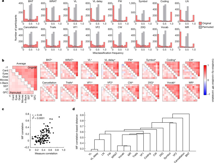
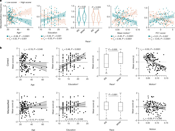
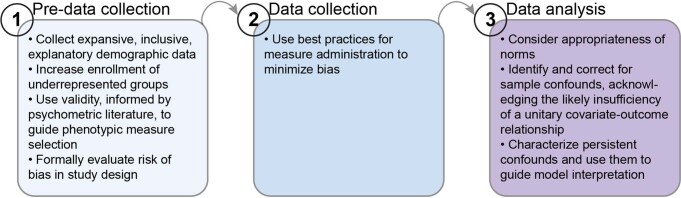
Individual differences in brain functional organization track a range of traits, symptoms and behaviours^1-12. So far, work modelling linear brain-phenotype relationships has assumed that a single such relationship generalizes across all individuals, but models do not work equally well in all participants^13,14. A better understanding of in whom models fail and why is crucial to revealing robust, useful and unbiased brain-phenotype relationships. To this end, here we related brain activity to phenotype using predictive models-trained and tested on independent data to ensure generalizability¹⁵-and examined model failure. We applied this data-driven approach to a range of neurocognitive measures in a new, clinically and demographically heterogeneous dataset, with the results replicated in two independent, publicly available datasets^16,17. Across all three datasets, we find that models reflect not unitary cognitive constructs, but rather neurocognitive scores intertwined with sociodemographic and clinical covariates; that is, models reflect stereotypical profiles, and fail when applied to individuals who defy them. Model failure is reliable, phenotype specific and generalizable across datasets. Together, these results highlight the pitfalls of a one-size-fits-all modelling approach and the effect of biased phenotypic measures^18-20 on the interpretation and utility of resulting brain-phenotype models. We present a framework to address these issues so that such models may reveal the neural circuits that underlie specific phenotypes and ultimately identify individualized neural targets for clinical intervention.

Fig. 1. FC can be used to classify scores on a range of neurocognitive measures.

a, Schematic illustration of the main classification pipeline. Classification was performed using leave-one-out (LOO) cross-validation. The training set was subsampled from the remaining participants to balance classes and was submitted to a linear support vector machine (SVM), using summed FC of selected edges as features. This trained model was then applied to the left-out test participant to classify their score as high or low from their FC. Participants who were successfully classified are termed ‘correctly classified participants’ (CCP), and participants who were misclassified are termed ‘misclassified participants’ (MCP). This procedure was repeated iteratively, with each participant used as the test participant, and this, in turn, was repeated 100 times with different training set subsamples selected on each iteration. This pipeline was repeated for each in-scanner condition and neurocognitive measure (numbers correspond to Yale study; comparable approach for UCLA and HCP). To ensure that the results are robust to these choices, analyses were repeated with alternative algorithms (bagging and neural networks); with 10-fold cross-validation; with an alternative parcellation of functional magnetic resonance imaging (fMRI) data; with an alternative threshold for score binarization; and with continuous phenotypic measures. See Methods, Extended Data Fig. 1 and Supplementary Table 11 for comparable results. b, Classification accuracy for each phenotypic measure, shown separately for high and low scorers and compared to the distribution of accuracy from 100 iterations of permutation tests (‘perm’). Significance was determined using the fraction of iterations on which the null classifier performed as well as or better than the median accuracy of unpermuted classifiers (across the whole sample) and resulting one-tailed P values were adjusted for multiple comparisons using the false discovery rate (FDR; 16 tests). Distributions and significance testing reflect accuracy across iterations for the best-performing in-scanner conditions, each noted in the plot title. For abbreviations and more on tasks and phenotypic measures, see Supplementary Tables 1 and 2. For sample sizes, see Supplementary Table 4. Source data

Fig. 2. Misclassification is consistent and phenotype specific.

a, Histogram of misclassification frequency for each phenotypic measure. Each histogram represents misclassification frequency (MF) for each participant, concatenated across in-scanner conditions and presented for analyses using original (that is, unpermuted) data (red) and permuted data (grey). b, Condition-by-condition correlation of misclassification frequency for analyses using original (top triangle) and permuted (bottom triangle) data, presented for each phenotypic measure. Condition order for individual phenotypic measures as in ‘Average’. *Significantly different from permuted result correlations, by paired, one-tailed Wilcoxon signed-rank test; all P < 0.0001, FDR adjusted (16 tests). r1, rest 1; r2, rest 2; GFC, general FC; grad, gradCPT. c, Relationship between phenotypic measure similarity (Spearman correlation) and misclassification frequency similarity (Spearman correlation). Each point represents a measure pair (given different participants excluded for intermediate, missing or outlier scores for each measure; number of correlated participants for each measure pair ranges from misclassification frequency: 63 to 114, measure: 105 to 129). d, Alternative visualization of misclassification frequency similarity, using a hierarchical linkage tree to reveal that measures that tap into similar constructs yield similar sets of misclassified participants. Source data

Fig. 3. Misclassification generalizes to an independent dataset.

a, For each of the three measures common to both datasets (LN, MR, vocabulary), six models were trained: one using all Yale participants (training set n: 80, 58, 58 for LN, MR, vocabulary, respectively), one using Yale CCP (50, 40, 40), one using Yale MCP (30, 18, 18), one using all UCLA participants (100, 78, 74), one using UCLA CCP (64, 48, 50) and one using UCLA MCP (36, 30, 24). Each model was applied to all high and low scorers in the test dataset (see Supplementary Tables 4 and 5 for test-set sizes), and the results are displayed as accuracy in all test participants, only in test CCP (Test: Correct), and only in test MCP (Test: Misclassified). *Significantly different from chance (mean accuracy using permuted data; dotted line presented for visualization only) by two-tailed, nested ANOVA; all P < 0.0001, FDR adjusted (nine tests). Bar height, grand mean; error bars, s.d. b, Similarity of model pairs, with similarity = 1 − Jaccard distance, thresholded at P < 0.05, by the hypergeometric cumulative distribution function. Models are divided into edges that are positively and negatively correlated with phenotype to facilitate interpretation. Larger, darker circles indicate increased similarity. Number of edges in each model (that is, selected on at least 75% of iterations): 30–374. Cells shaded on the basis of predicted patterns of similarity. c, Each model’s highest-degree node and its incident edges are visualized in all models. Models for which the depicted node is the highest-degree node are enclosed in grey rectangles. Red, positive relationship with phenotype; blue, negative relationship with phenotype. Node size scales with degree, and nodes are coloured red if, of the edges incident to that node, the number of edges positively related to phenotype is greater than or equal to the number of edges negatively related to phenotype; blue otherwise. P, edges positively correlated with phenotype; N, edges negatively correlated with phenotype; UM, Yale MCP train, UCLA test; UC, Yale CCP train, UCLA test; YC, UCLA CCP train, Yale test; YM, UCLA MCP train, Yale test. Node number in the Shen atlas (MNI coordinates). Source data

Fig. 4. Frequently misclassified participants defy stereotypical profiles.

a,b, Data are shown for all covariates that were found to have significant pairwise relationships with misclassification frequency by two-tailed rank correlation and Mann–Whitney U test. a, Relationship with misclassification frequency, averaged separately across measures on which participants scored high (‘high scorer’) and low (‘low scorer’). *Significant (P < 0.05) in corresponding full regression of low- or high-scorer misclassification frequency on these covariates. b, Relationship with mean scores, averaged separately across measures on which participants were frequently correctly (top) and incorrectly (bottom) classified. *Significant (P < 0.05) in full regression of mean (correct or misclassified) score on these covariates. Lines and shading: best-fit line from simple linear regression with 95% confidence bands. Violin plot lines represent median and quartiles. Box plot centre line and hinges represent median and quartiles, respectively; whiskers extend to most extreme non-outliers. All reported P values FDR adjusted (a, 30 tests; b: 8 tests). See Supplementary Tables 9 and 10 for relationships between misclassification frequency, mean score and all tested covariates, as well as sample sizes. RG, racialized groups. Source data

Extended Data Fig. 1. Model performance and misclassification frequency are robust to analysis approach.

(a) Classification accuracy for each phenotypic measure using FC calculated from all in-scanner conditions in the Yale dataset, and five different analysis pipelines: an alternative, 368-node parcellation for FC matrix generation, two alternative classification algorithms (ensemble of weak learners and neural network), an alternative phenotypic binarization threshold (mean split), and an alternative (10-fold) cross-validation approach (see Methods for additional description of each analysis). Box plot line and hinges represent median and quartiles, respectively; whiskers extend to most extreme non-outliers; outliers plotted individually (+). Number of classified individuals and size of training sample same as in main analyses (see Supplementary Table 4) for all analyses except mean split (4 measures [see below], number classified = 109-127, training sample size = 72-82) and 10-fold (number classified same as in main analyses, training sample size = 34-110). r1, rest 1; r2, rest 2; grad, gradual-onset continuous performance task; sst, stop signal task; gfc, general FC. (b) Misclassification frequency (MF), averaged across in-scanner conditions and phenotypic measures to derive a single value per participant, compared between each alternative analysis and main-text analyses. r_s, two-tailed rank correlation, n = 128-129, P values FDR adjusted. Note that phenotype mean split is equivalent to mean ± 1/3 × s.d. for scaled scores; mean split-based model accuracy is not reported for these measures, nor are they included in the calculation of misclassification frequency. Given the limited mean split-based results, we repeated this analysis in the HCP data, with comparable results (mean misclassification frequency r_s = 0.86, P < 0.0001). 10-fold results reflect 1,000 analysis iterations per phenotypic measure and in-scanner condition (50 per cross-validation partition); all other analyses reflect 100 iterations. In this and all subsequent figures: BNT, Boston Naming Test; WRAT, Wide Range Achievement Test; VL, verbal learning; FW, finger windows; LN, letter–number sequencing; Trails, trail making; VF, verbal fluency; CW, colour–word interference; 20Q, 20 questions; Vocab, vocabulary; MR, matrix reasoning.

Extended Data Fig. 2. Replication of classification and internal validation results in the UCLA CNP dataset.

Results as presented in Fig. 1b, Fig. 2, and Fig. 4a. (a) Significance via one-tailed permutation testing (as in Fig. 1b); P values FDR adjusted (3 tests). For sample sizes, see Supplementary Table 5. (b) As in Yale data, mean of permuted distribution did not significantly differ from 0.5 (all P > 0.05, FDR adjusted [3 tests]), mean and median of original data-based distribution significantly differed from 0.5 (all P < 0.0001, FDR adjusted [6 tests] via two-tailed t- and Wilcoxon signed-rank tests), and the misclassification frequency distributions for original and permuted analyses significantly differed for each measure (all P < 0.0001, FDR adjusted [3 tests] via two-tailed, two-sample Kolmogorov–Smirnov test). (c) *P < 0.0001, FDR adjusted (3 tests) via paired, one-tailed Wilcoxon signed-rank test (as in Fig. 2b). (d) Given the small number of included measures, we present these results only for consistency with main analyses. As in Fig. 2c, different participants excluded for intermediate, missing, or outlier scores for each measure; number of correlated participants for each measure pair ranges from misclassification frequency: 103-138, measure: 162-163. (e) Results as presented in Fig. 4a. Covariate relationships presented if they were significantly related to misclassification frequency in low or high scorers (P < 0.05, adjusted), or if they were significantly related to misclassification frequency in Yale analyses (education, race) to demonstrate comparable trends. All P values FDR adjusted (22 tests). For full results and relationship of covariates to mean score, as well as sample sizes, see Supplementary Tables 9 and 10. PAMret, paired associates memory task, retrieval; SST, stop signal task; MF, misclassification frequency.

Extended Data Fig. 3. Replication of classification, internal validation and external validation results in the HCP dataset.

Results as presented in Fig. 1b, Fig. 2a, b, Fig. 3a, and Fig. 4a. Given the large HCP sample size, 10-fold cross-validation was used (20 partitions, 50 subsampling iterations each), with the requirement that family members be assigned to the same fold. Given that only two measures were classified, we omit measure versus misclassification frequency similarity and hierarchical linkage analyses. (a) Significance via one-tailed permutation testing (as in Fig. 1b); P values FDR adjusted (2 tests). For sample sizes, see Supplementary Table 6. (b) Permuted distribution means significantly differed from 0.5 via two-tailed, one-sample t-test (cIQ mean = 0.491 [P < 0.0001], fIQ mean = 0.498 [P = 0.04], both FDR adjusted [2 tests]). All else as in Yale and UCLA analyses: mean and median of original data-based distribution significantly differed from 0.5 (all P < 0.0001, FDR adjusted [4 tests] via two-tailed t- and Wilcoxon signed-rank tests), and the misclassification frequency distributions for original and permuted analyses significantly differed for each measure (all P < 0.0001, FDR adjusted [2 tests] via two-tailed, two-sample Kolmogorov–Smirnov test). MF, misclassification frequency. (c) **P = 0.001, ****P < 0.0001, FDR adjusted (2 tests) via paired, one-tailed Wilcoxon signed-rank test (as in Fig. 2b). (d) Results presented as in Fig. 3a. Bar height, grand mean; error bars, s.d. *P < 0.0001, FDR adjusted (9 tests) via two-tailed, nested ANOVA. For each classified measure (cIQ/vocabulary and fIQ/MR for HCP/Yale), six models were trained: 1 using all Yale participants, 1 using Yale CCP, 1 using Yale MCP (see Fig. 3 legend for training set sizes), 1 using all HCP participants (number of participants used for training after excluding intermediate and outlier scores and subsampling to balance classes: 230 and 350 for crystallized and fluid measures, respectively), 1 using HCP CCP (168, 216), and 1 using HCP MCP (62, 134). See Supplementary Tables 4 and 6 for test-set sizes. (e) Results as presented in Fig. 4a. Covariate relationships presented if they were significantly related to misclassification frequency in low or high scorers (P < 0.05, adjusted). For full results and relationship of covariates to mean score, as well as sample sizes, see Supplementary Tables 9 and 10. ****P < 0.0001; all P values FDR adjusted (22 tests).

Extended Data Fig. 4. Selected edges for top-degree nodes in each Yale/UCLA model.

Results as presented in Fig. 3c. For MR, YM and Vocabulary, UC two nodes were tied for highest degree (MR, YM: 26 and 157; Vocabulary, UC: 166 and 191). Only one node for each model visualized for illustration.

Extended Data Fig. 5. Comparison of FC between CCP and MCP groups at edge and network levels.

Edges, GFC: t statistics for each GFC edge found to significantly differ (via two-sample t-test) between groups (P < 0.05, FDR adjusted), ordered by network. Red, CCP>MCP; Blue, MCP>CCP. Networks, GFC: mean t statistics for each network pair (using GFC) found to significantly differ (via Constrained NBS) between groups (one-tailed P < 0.025, FDR adjusted). Red, CCP>MCP; Blue, MCP>CCP. Significant edges across tasks and Significant networks across tasks: Number of times (i.e., tasks for which) edge (ordered by network) or network pair was significantly greater for CCP than MCP – number of times edge or network pair was significantly greater for MCP than CCP. Mean GFC, CCP and Mean GFC, MCP: GFC, averaged across participants within each group; main diagonal set to 0, and nodes ordered by network. Note that CCP and MCP groups differ for each phenotypic measure and in-scanner task (range of number of participants using GFC across phenotypic measures: CCP = 46-81, MCP = 23-63). Black dashed lines separate networks: 1 = medial frontal, 2 = frontoparietal, 3 = default mode, 4 = motor, 5 = visual A, 6 = visual B, 7 = visual association, 8 = salience, 9 = subcortical, 10 = cerebellum (for network visualization, see).

Extended Data Fig. 6. Future directions.

Schematic representation of recommended framework for study design and analysis to yield more precise, useful, and unbiased models.

Extended Data Fig. 7. Race and ethnicity.

Reported racial and ethnic breakdowns of the Yale, UCLA and HCP samples.

References

1. Finn ES, et al. Functional connectome fingerprinting: identifying individuals using patterns of brain connectivity. Nat. Neurosci. 2015;18:1664–1671. - PMC - PubMed
1. Dubois J, Galdi P, Paul LK, Adolphs R. A distributed brain network predicts general intelligence from resting-state human neuroimaging data. Philos. Trans. R. Soc. B. 2018;373:20170284. - PMC - PubMed
1. Rapuano KM, et al. Behavioral and brain signatures of substance use vulnerability in childhood. Dev. Cogn. Neurosci. 2020;46:100878. - PMC - PubMed
1. Drysdale AT, et al. Resting-state connectivity biomarkers define neurophysiological subtypes of depression. Nat. Med. 2016;23:28–38. - PMC - PubMed
1. Hsu W-T, Rosenberg MD, Scheinost D, Constable RT, Chun MM. Resting-state functional connectivity predicts neuroticism and extraversion in novel individuals. Soc. Cogn. Affect. Neurosci. 2018;13:224–232. - PMC - PubMed