Constructive connectomics: How neuronal axons get from here to there using gene-expression maps derived from their family trees

Abstract

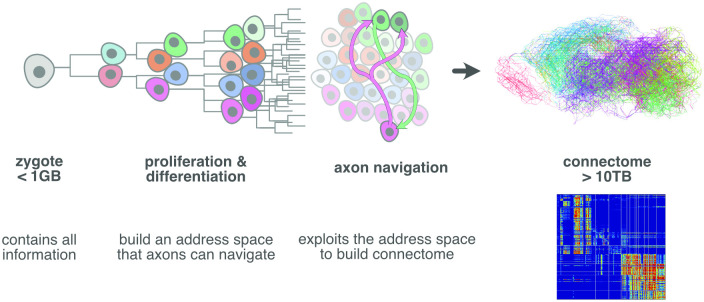
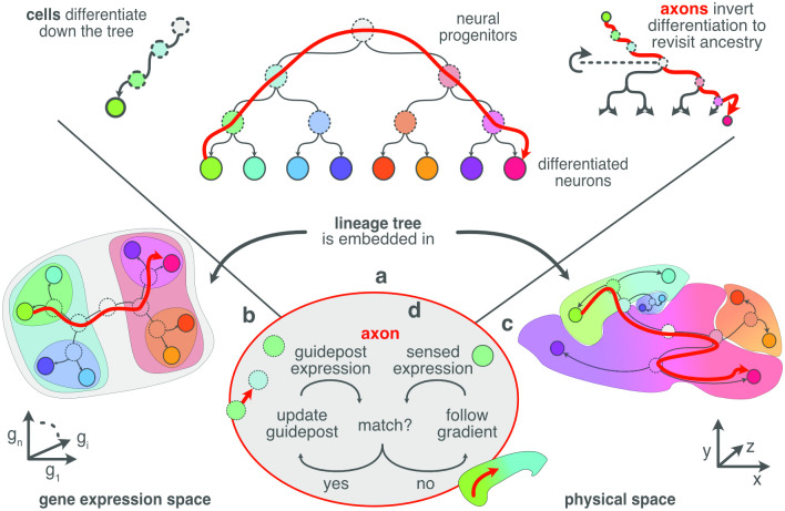
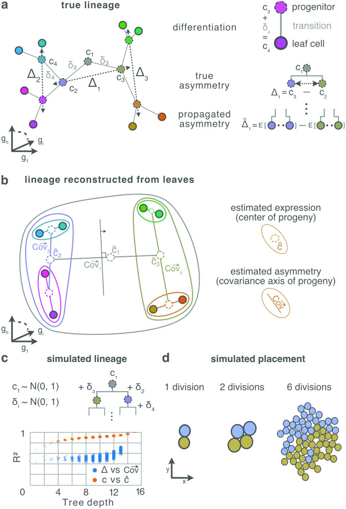
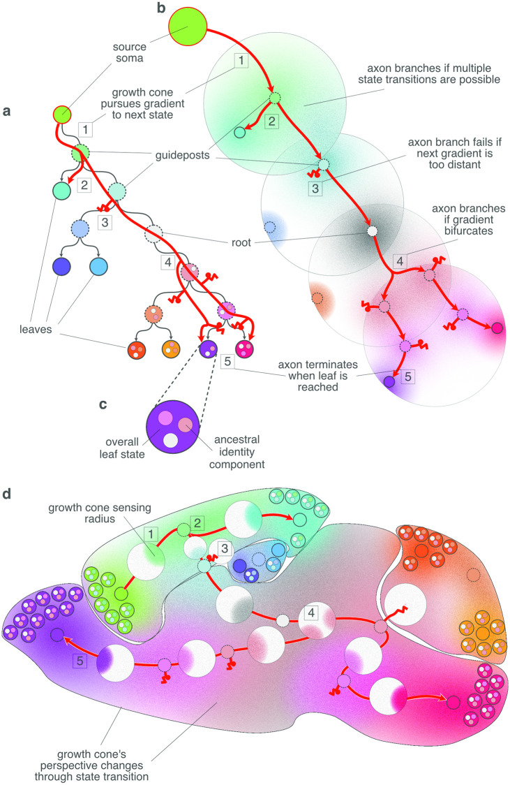
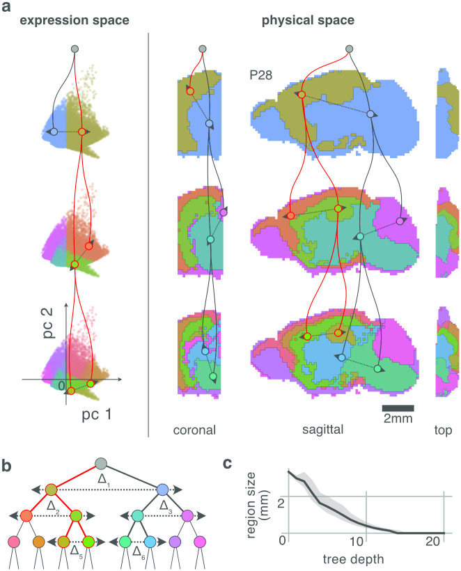
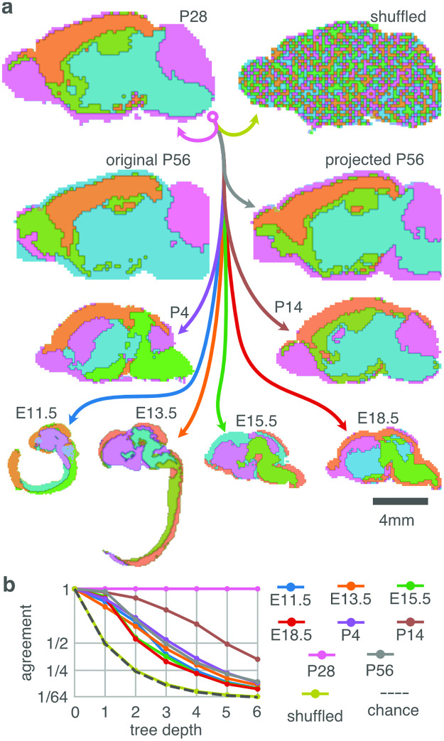
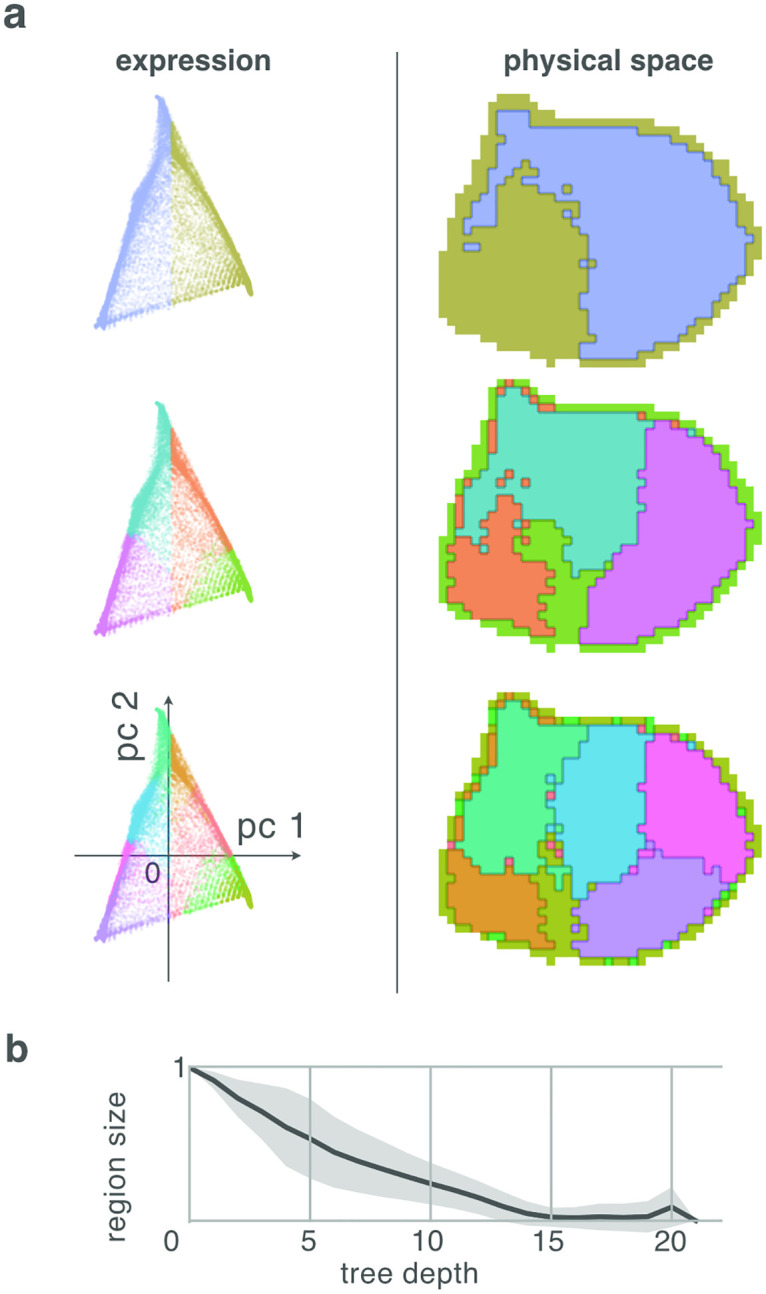
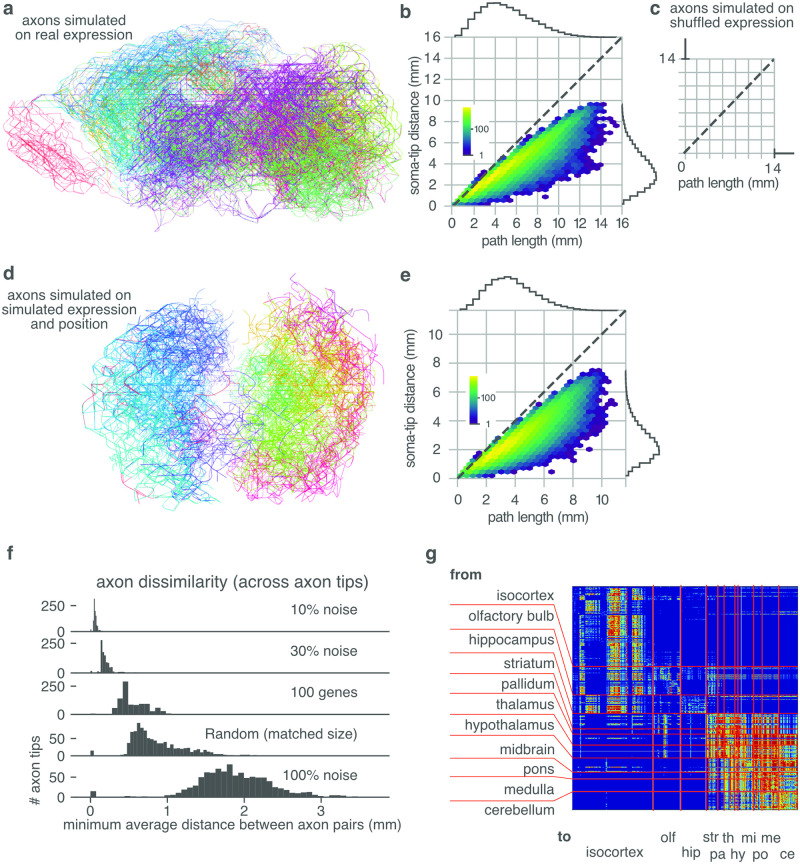
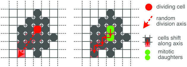
During brain development, billions of axons must navigate over multiple spatial scales to reach specific neuronal targets, and so build the processing circuits that generate the intelligent behavior of animals. However, the limited information capacity of the zygotic genome puts a strong constraint on how, and which, axonal routes can be encoded. We propose and validate a mechanism of development that can provide an efficient encoding of this global wiring task. The key principle, confirmed through simulation, is that basic constraints on mitoses of neural stem cells-that mitotic daughters have similar gene expression to their parent and do not stray far from one another-induce a global hierarchical map of nested regions, each marked by the expression profile of its common progenitor population. Thus, a traversal of the lineal hierarchy generates a systematic sequence of expression profiles that traces a staged route, which growth cones can follow to their remote targets. We have analyzed gene expression data of developing and adult mouse brains published by the Allen Institute for Brain Science, and found them consistent with our simulations: gene expression indeed partitions the brain into a global spatial hierarchy of nested contiguous regions that is stable at least from embryonic day 11.5 to postnatal day 56. We use this experimental data to demonstrate that our axonal guidance algorithm is able to robustly extend arbors over long distances to specific targets, and that these connections result in a qualitatively plausible connectome. We conclude that, paradoxically, cell division may be the key to uniting the neurons of the brain.

Fig 1. The connectome is the result of a constructive process that starts ultimately with the zygote, and involves the two aspects of first generating a mass of cells with various types, and then routing axons through this mass to their proper targets.

An observer’s description of the resulting detailed mouse connection matrix (right bottom) takes at least 10 TB to encode. However, as development occurs largely in isolation, all instructions to construct this connectome must fit through the narrowest part of the bottleneck of inherited information: i.e., the zygotic genomic sequence. This implies that neural progenitors have efficient methods for expanding the highly compressed wiring instructions into axonal trajectories. To do this, they need to, as they proliferate and differentiate, install a space of molecular addresses that axons can exploit for navigation.

Fig 2

As progenitors divide they progressively differentiate their gene expression until they reach their post-mitotic neuronal states at the leaves of the lineage tree (A: top left). Constraints on mitosis (see text) embed the global neuronal lineage tree (A) into both gene expression (B) and physical space (C), so that cells of related differentiation have similar expression profiles (similar colors) and are nearby one another physically. Consequently, a trajectory from one leaf node to another through the lineage tree (A: red arrow) often corresponds to an unbroken trajectory through both gene expression space (B: red arrow) and physical brain space (C: red arrow). An axon navigates by inverting its source neuron’s instance of the global genetic differentiation program (A: top right). This inversion generates a sequence of expression profiles that correspond to ancestral states and so act as guidepost profiles. D The axonal branch configures its growth cone to match the sensed expression to the internally generated expression, and so moves to the direction that improves that match. When the match can no longer be improved by moving, the axon updates its internal state to the next ancestor, and repeats. If the match between internal and external expression can be improved by moving into multiple different directions, or by transitioning to multiple different states, the single axonal branch is split into two new branches that continue to execute the same algorithm, but whose independent states may subsequently diverge. When an axonal branch arrives at a leaf state, both in expression and physical space, navigation of that branch is complete and local synapses are formed.

Fig 3

A Cells are points positioned in high-dimensional expression space, where each axis represents the expression of one gene. Here, this high-dimensional space is reduced to 2D dimensions for plotting purposes, so that their 2D distance approximates their high-dimensional distance. In our division model, the differential expression between a parent cell c₁ and its daughters c₂, c₃ is a normally distributed random vector representing the genetic state transition from parent to daughter, denoted δ₂ = c₂ − c₁. (Here we use the division of the root progenitor 1 as a running example for any division.) The differential expression between two siblings, which we call the parent’s asymmetry, is denoted Δ₁ = c₃ − c₂ = δ₃ − δ₂. As a result, the correlation in gene expression between two cells reflects their distance through the lineage tree. (See C for verification of this process by numerical simulation.) B The expression of a progenitor can be estimated as the mean expression over its leaf progeny; and the asymmetry of a progenitor can be measured as the main axis of variance across its progeny. The diagram shows only the leaves of the lineage tree show in A—they have identical positions in embedded expression space. Each nested contour encloses the progeny of a progenitor; lines within the contour indicate the main axis of variance across the enclosed progeny; and dotted circles the average expression across the progeny. The sets of progenies for individual progenitors can be obtained by iteratively splitting the progeny along their main axis of variance, so with a decision boundary (black line with arrow) orthogonal to this axis. C Numeric simulation of expression profiles induced by our division model, and subsequent reconstruction of expression profiles and mitotic asymmetries from the leaves of the simulated tree. The root expression c₁ is drawn from a normal distribution with zero mean and unit variance. The expression profiles of other cells are generated recursively by adding differential expression patterns δ_i, which are also normally distributed. (All random number are drawn independently.) The determination (squared correlation) was measured between the true and reconstructed asymmetries (blue), and true and reconstructed expressions (orange). D Progenies group naturally in brain space according to their ancestry. Shown is a 2D simulation of growing tissue, started from a single root, only constrained to not detach from one another and not pass through each other.

Fig 4. Navigation of an axon (red branching arrow) through the familial address space.

Throughout the figure, similarity in color denotes similarity in gene expression profile. A The axon traverses the brain by traversing a sequence of familial states of the lineage tree that is implicit in its genome. The growth cone uses the sequence of familial states as successive search templates in brain space, and so navigates from a source leaf node to a number of target leaves. Familial states (colored circles) correspond to nodes of the encoded lineage tree. For purpose of explanation, the tree is hung from the leaf state corresponding to the axon’s source neuron, rather than from its root node as in Fig 3b. Terminal states of leaf (existent) nodes have a solid circumference, while ancestral states in the interior of the tree have a dotted circumference. Transitions between states occur downward, along the arrowed arcs, beginning at the source leaf (red encircled) and ending at (some) other leaves. The original tree root can be recognized as the only state having two edges, rather than three (since the root progenitor has no mitotic parent). B Various decision scenarios that the axon encounters during traversal. Each familial state is characterized by a profile of gene expression, whose distribution across all cells peaks at one or more locations in brain space. The gradient of a state in the familial address space is the frequency of encountered cells that test positively for a familial state. By selecting a particular familial template, the growth cone tunes into the corresponding expression gradient and filters out the others. If the tuned gradient is in range, the growth cone follows it to arrive at one of that gradient’s peaks (case indicated by $\boxed{1}$). If the tuned gradient is not in range $\boxed{3}$, the axonal branch of that growth cones fails. When the axon arrives at a peak, its growth cone tunes to the next downstream familial state, and so on, until a leaf state is found. If multiple downstream states are in range, the axon branches $\boxed{2}$, with each branch tuned to one of the possible downstream states. The axon also branches if the gradient is bifurcated by a valley, so that the axon can follow an upward gradient in multiple directions $\boxed{4}$. Each branch pursues a different direction, but in this case they are tipped with growth cones in the same state (unlike the branches in scenario $\boxed{2}$). When a growth cone reaches a leaf state, guidance terminates $\boxed{5}$. C Cells have composite genetic identities, with one component (small inner circle) inherited from each ancestor state. The overall state of a leaf cell is the aggregation of these components (Fig 3). A growth cone can test whether a cell possesses a component by selecting the familial state template corresponding to that component, and then matching the internally produced gene expression to that of the tested cell. D Various regions of the brain correspond to branches of the mitotic lineage tree. Consequently, the regions are nested and each marked by the component of the genetic identity code corresponding to the common progenitor of the region.

Fig 5. Hierarchical decomposition of covariance in gene expression space brain is mirrored by a matching decomposition in brain space.

Here the results are for postnatal (P) day 28. The results from further time points can be found in S3–S10 Figs. A Expression Hierarchical decomposition on the collection of voxels in expression space, independent of source location in brain. Decomposition is performed by measuring the first principal component of covariance; then sorting all voxels into two bins, (competing bins indicated by dotted arrows) based on their individual projection coefficients. This process is repeated recursively on each of the resulting bins, until a bin contains only a single voxel remains (Figure shows only the first 3 generations of the resulting hierarchy). Physical Space Same voxel bins and coloring, but voxels now positioned at their source locations in brain. Coronal and horizontal sections are shown: the color of each pixel indicates the most common bin in the occluded direction for that pixel. Horizontal section (labeled top) is drawn at a smaller scale. Multiscale spatially coherent covariance patterns are present. Two example branches of the hierarchy are indicated with red and black curves. B Hierarchy of bins of the hierarchical decomposition. The bins are colored to represent the hierarchy: the parent bin has the average hue of the child bins. This coloring is applied throughout the paper. C Although regions are nested by construction (hierarchical decomposition), we quantified the extent to which the regions are also continuous by measuring their spatial spread (average distance from the region centroid) as a function of their depth in the hierarchy. At the root of the hierarchy the spatial spread covers the entire brain, and we expect that as the depth increases the spatial spread (i.e., the mean distance from the region centroid to the constituent voxels) decreases. To make the different time points and simulation comparable we present the spreads as a fraction of the root spread. The solid line indicates the median spread over all regions at that depth, and the gray area the first (below) and third (above) quartiles. As expected, the mean distance from the centroid decreases as the regions become more resolved with depth.

Fig 6. The root asymmetry measured at P28 is projected to the other available embryonic and post-natal developmental time points, and compared to the root asymmetry measured at the respective time point.

A First division of the hierarchy, but the direction of variance used to sort the bins is derived from P28, rather than from the data of the time point itself (except Original P56). This temporally projected pattern only has small differences with the patterns derived from the original data (compare Original P56 to Projected P56). When the expression data is shuffled over voxels and genes, maintaining pooled expression statistics but destroying covariance structure, all spatial patterning disappears. Images are proportional to their actual brain sizes. B Quantification of the agreement between the original and projected hierarchy, measured as the proportion of voxels in matching bins, at different levels in the hierarchy. (Although the images in A are 2D, quantification is done on the 3D voxels.) The number of possible bins grows exponentially with tree depth, and so chance level decreases inverse-proportionally (dashed line), quantitatively verified by the shuffled case (yellow line). P28 projects onto itself, and is hence in perfect agreement. The other time points show an agreement consistently above chance. Consider that a mismatch at a shallow depth cannot be corrected at a deeper depth, and so mismatch can only accumulate.

Fig 7. Random sets of genes of various sizes from embryonic age E11.5 were selected, and the spatial hierarchy they exhibit was compared to the hierarchy exhibited by the grand set of all genes at hierarchy.

To compare hierarchies all voxels are projected onto both hierarchies. For each matching choice the score is incremented proportionally to the depth of the bin. As such, 1 indicates that the all voxels are sorted into corresponding nodes of the hierarchies, and the dotted line indicates the score if all voxels were sorted into hierarchical bins randomly (as in the shuffled case). The hierarchy established from a set of 20 random genes already agrees largely above chance with the original pattern. Black dots represent the accuracy from the data at E11.5. Blue dots indicate the same experiment, but on shuffled expression data.

Fig 8. Hierarchical decomposition of expression data generated by simulation of the model (see text) proposed to explain the results.

Simulated ‘brain’ sphere composed of voxelated leaf cells was generated by 300,000 mitoses distributed over 10 independent lineages. Cells express 500 genes. Asymmetrical mitoses induce differential changes in gene expression. Each voxel contains 3 × 3 × 3 = 27 adjacent cells. Similar to experimental results, the hierarchical decomposition of covariance in gene expression voxels independent of location (left), is mirrored by matching decomposition in space (right).

Fig 9. Simulated axons use familial guidance to navigate through the voxels of the ABI developing mouse brain gene expression atlas.

A Arborizations of 50 example axons, show in a sagittal projection of the ABI atlas hemisphere. Each arbor is the collection of all branches that an axon could potentially navigate using this gene expression space. Each axon is colored according to its source region. The colors correspond to those of Fig 5B. B Straight-line distance between the beginning of a branch (soma) and end of that branch (top) versus the actual path length. Branches are points sorted in hexagonal 2D bins, whose color intensity indicates the number of branches in that bin. C Same as B, but expression values are shuffled before the hierarchical decomposition and axon guidance algorithm are applied. In this control case guidance fails completely, and no axons cannot guide outside their original voxel. D Arborizations of 50 example axons using the same algorithm as in A, but on tissue grown in simulation (as in Fig 8). E As B, but for the simulated tissue of D. F The dissimilarity, measured as the average minimum distance between axon tips, between simulated axons on experimental expression (as in A). Axons begin from the same voxel, but are under varying levels (10%–100%) of expression noise; or guide using only a subset of 100 genes selected randomly (i.e., the same 100 genes are used for all simulated axons). Because the navigation algorithm is deterministic the 0% noise case produces identical neurons. The familial guidance dissimilarity is compared against a random walk axon of the same path length. G Connectivity matrix corresponding to the connections made by the axons of A. The connection patterns are block-structured and adhere to known anatomical boundaries. The anatomical regions marked on the matrix are taken from the annotations of the Allen Institute for Brain Science. The anatomical annotations were not used during simulation.

Fig 10. Illustration of cell placement.

Although the illustration is 2D, the placement is the same for 3D. When a cell divides a random division axis is drawn uniformly from a unit circle (in 2D) or sphere (in 3D). Then, the sequence of cells that intersect the division axis are shifted along the sequence to create a free slot next to the dividing cell. The mitotic daughters take the original slot of the parent, and the newly created free slot.