Multiscale fluorescence imaging of living samples

Abstract

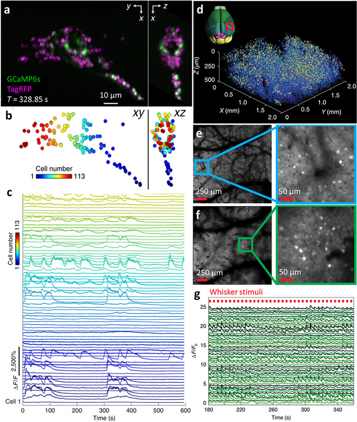
Fluorescence microscopy is a highly effective tool for interrogating biological structure and function, particularly when imaging across multiple spatiotemporal scales. Here we survey recent innovations and applications in the relatively understudied area of multiscale fluorescence imaging of living samples. We discuss fundamental challenges in live multiscale imaging and describe successful examples that highlight the power of this approach. We attempt to synthesize general strategies from these test cases, aiming to help accelerate progress in this exciting area.

Keywords: Fluorescence; Live imaging; Microscopy; Multiscale.

Fig. 1

Multiscale imaging spans diverse spatiotemporal scales, which are usually accessed via distinct microscopy modalities. a Examples of biological phenomena that occur over the nanometer to centimeter spatial scale, and over timescales ranging from milliseconds to days. Note that rapid motion (here indicated by rates) occurs at all scales. b Typical fluorescence microscopy methods used in living samples over indicated spatiotemporal scales. Note that boundaries between methods are ‘fuzzy’ and only approximate

Fig. 2

Basic considerations and tradeoffs in multiscale imaging. a Trading field of view (FOV) for spatial resolution. Images of DAPI-stained nuclei in fixed U2OS cells acquired with widefield microscopy. Insets show higher-magnification views of a single nucleus. Left: image acquired with 20x/0.5 NA dry objective lens; Right: image of a different field of view acquired with a 60x/1.42 NA oil immersion objective lens. A larger field of view (FOV) can be attained by using an objective with lower magnification, albeit with worsened spatial resolution. b Larger pixels compromise spatial resolution, but improve SNR. Images of GFP-histone-labeled C. elegans embryos acquired with light sheet microscopy (Wu et al. 2017). Left: with a pixel size of 130 nm; Middle: after digitally binning pixels to 390 nm to mimic the case when detector with larger pixels is used. Right: Intensity profiles over the yellow lines in images, showing improved SNR with larger pixel size. Larger pixels are sufficient to image coarser features (e.g., nuclei), but fine features within nuclei, evident during cell division (red arrows) are better resolved with a smaller pixel size. c Motion blur due to insufficient temporal resolution. Images of mitochondria (green) and lysosomes (red) in human colon carcinoma (HCT-116) cells, acquired with multiview confocal microcopy (Wu et al. 2021). Left: maximum intensity projection in lateral view at a typical time point; Middle: magnified view of the white rectangle in the most left column, acquired at rate of ~ 2 s per volume; Right: same as in the middle column, but acquired at rate of ~ 1 s per volume, showing four time points. Rapidly moving lysosomes (magenta arrow) are blurred at slower imaging rate, and better resolved when imaging at a faster rate (white arrows). Motion blur is less problematic at larger length scales (orange arrows)

Fig. 3

Multiscale imaging by combining distinct microscopy modalities. a STED, PALM, and µPAINT enable imaging of molecular trajectories within the context of super-resolved dendritic spines in a living hippocampal neuron. b Magnified view of two spines from the overlay image in (a), showing GluA1_SEP AMPA receptor trajectories inside and outside the PSD95 area, as well as freely moving along dendrites and spinules (white arrows). Individual trajectories are shown as distinct colors. c, d 3D reconstruction of a single vesicular stomatitis virus (VSV)-G pseudotyped lentiviral vector particle trajectory, as it ‘skims’ along the surface of live HeLa cells. The particle trajectory and cell morphology were simultaneously interrogated by combining 3D tracking and imaging (3D-TrIm), integrating real-time active-feedback tracking microscopy with a volumetric imaging system. Cells are color-coded by intensity and distance from the cell surface to the virus trajectory in (c) and (d), respectively. Circular inset: enlarged view of “skimming” event. e XY view with trajectory superimposed. f YZ view of the same cell and trajectory, with trajectory color-coded according to diffusion coefficient. a, b were reprinted with permission from ref (Krishna Inavalli et al. 2019), and c–f reprinted with permission from ref (Johnson et al. 2021)

Fig. 4

Rapid multi-scale functional imaging in living organisms. a Lateral (left) and axial (right) maximum intensity projections highlighting nerve ring region from a living, immobilized C. elegans young adult (NLS-GCaMP6s/TagRFP), acquired with SCAPE 2.0 at 5.96 volumes per second. b 113 neurons were identified and tracked in 3D space over 10 min and are ordered and color-encoded along the rostral-caudal axis. c Extracted raw GCaMP6s fluorescence time courses over 10 min. d Volumetric imaging (spanning ~ 2 × 2 × 0.5 mm³) of neural activity at 6.7 Hz in jGCaMP7f-expressing mice, acquired with light beads microscopy. 3D rendering of extracted neuron spatial coordinates and maximum projected activity for a 9-min recording. The red rectangle in the transverse brain image indicates the region over which responses from 70,275 neurons were recorded. e, f Mean projection images at 144- and 482-μm depths, respectively, with higher magnification views at right. g Representative time series of 50 whisker-tuned neurons. Occurrences of the whisker stimulus are denoted by red marks. a–c were reprinted with permission from ref (Voleti et al. 2019), and d–g reprinted with permission from ref (Demas et al. 2021)

Fig. 5

Adaptively correcting for sample size and aberrations when using light-sheet and three-photon microscopy improves imaging at large length scales. a Reconstruction of mouse embryo at single-cell resolution, acquired with adaptive light sheet microscopy. Three time points (hh:mm) selected from an experiment spanning mid/late-streak stage to early somite stage. Here, tracks are derived from combining the cell-tracking framework with a machine learning module (TGMM 2.0) and statistical vector flow (SVF) analysis. The dynamic fate map was created by labeling tissues in the image data at the last time point, transferring labels to SVF objects (spheres) and propagating labels backwards in time. b, c Tiled adaptive optics (AO) lattice light sheet microscopy permits detailed examination of cellular morphology and organelle distributions across the eye of a developing zebrafish embryo 24–27 h post fertilization. Here, computationally separated cells are shown spanning the data in (b), with organelles colored as indicated. Orthoslices at six different time points are shown in (c) highlighting cell divisions (white and green arrowheads, left panel) at the apical surface of the retinal neuro-epithelium and mitochondria (orange arrowheads) present from the apical to the basal surface in one dividing cell. d ECG-gated AO 3PM at 1300-nm excitation wavelength in EGFP–Thy1(M) mouse visual cortex and hippocampus, shown as 3D reconstruction of an image stack of third-harmonic signal (cyan) and GFP-labeled neurons (green). Aberration correction is performed via a modal-based indirect wavefront sensing approach. Intravital motion artifacts are reduced with a real-time ECG-gated image acquisition scheme that synchronizes scanners to the cardiac cycle of the mouse. e Maximum intensity projection of a neuron in the mouse cortex (Thy1-YFP-H), at 747–767 μm below dura, under 1300-nm three-photon excitation, without and with AO based on a zonal aberration measurement method. f Higher-magnification views of the red square in e, 751–767 μm below dura, without and with AO. Insets show higher magnification views of the dendrite shown in white rectangles in f. 10 × digital gain was applied to the No AO inset to increase visibility. Reprinted with permission from ref (McDole et al. 2018) for (a), ref (Liu et al. 2018) for (b, c), ref (Streich et al. 2021) for (d), and ref (Rodriguez et al. 2021) for (e, f)

Fig. 6

Image restoration with deep learning. a With suitable training data, a neural network may be used to denoise images. b Lateral (upper) and axial (lower) images of a fixed U2OS cells expressing mEmerald-Tomm20 imaged via iSIM, comparing noisy raw iSIM data acquired with low-intensity illumination (left), deconvolved GT data acquired with high-intensity illumination (middle), and RCAN output (right) given raw input. c RCAN denoising enables the collection of thousands of iSIM volumes without photobleaching. Mitochondria in live U2OS cells were labeled with pShooter pEF-Myc-mito-GFP and imaged with high- (360 W cm^–2) and low- (4.2 W cm^–2) intensity illumination. Top row: selected examples at high illumination power, illustrating severe photobleaching. Middle row: selected examples from a different cell imaged at low illumination power, illustrating low SNR (Raw). Bottom row: RCAN output given low SNR input. Numbers in top row indicate volume #. d The graph quantifies the normalized signal in each case in (c); ‘jumps’ in Raw and RCAN signal correspond to manual refocusing during acquisition. e–g Two-step RCAN process (RCAN denoising followed by RCAN expansion) is applied to deconvolved iSIM images to generate expansion predictions. Images from live U2OS cells expressing EGFP-Tomm20 were acquired with iSIM, deconvolved and input into the two-step RCAN process. e Overview of lateral and axial maximum intensity projections of first volume in time series from two-step RCAN prediction. f Higher-magnification views of red rectangular region in (e), comparing raw iSIM and RCAN prediction. Red arrows highlight mitochondria better resolved with RCAN than iSIM. g Higher-magnification views of axial slice corresponding to yellow rectangular region in (e), comparing deconvolved iSIM input (left) and two-step RCAN output (right). Yellow arrows highlight mitochondria that are better resolved with RCAN output than input data. h–j Super-resolution images of ER (magenta) and mitochondrial cristae (green) in live U2OS cells, acquired with GI-SIM and generated by DFCAN-SIM (ER) and DFGAN-SIM (mitochondria), respectively. Top right: a fraction of the corresponding widefield image averaged from raw SIM images. Time-lapse images showing mitochondrial fission (i) and fusion (j) events occurring at ER–mitochondria contact sites. k–n Deep learning and joint deconvolution produces 2D super-resolution images from diffraction-limited input. Example 2D SIM maximum intensity projection of U2OS cell expressing Lifeact tdTomato, volumes every 10 s, over 100 time points. Images are color-coded to indicate temporal evolution. l–n Comparative higher-magnification view of blue, yellow, red regions in (k), color-coded in (m, n) to illustrate the filopodial dynamics. Reprinted with permission from ref (Chen et al. 2021) for (a–g), ref (Qiao et al. 2021) for (h–j), and ref (Wu et al. 2021) for (k–n)

Fig. 7

Image-based event triggering improves multiscale imaging of fine dynamic processes. a Schematic for event triggered STED (etSTED): widefield calcium imaging of Oregon Green 488 BAPTA-1 in neurons, corresponding ratiometric images, detected events, and local etSTED images of SiR-tubulin. The green cross indicates the ratiometrically brightest detected event that triggered STED imaging and the red crosses indicate additionally detected events in the same widefield frame. b Timeline of typical etSTED experiment, with widefield, analysis pipeline, overhead, and STED imaging time indicated. c etSTED experiments, imaging protein synaptotagmin-1(syt-1) conjugated to Abberior STAR635P. Syt-1 is the calcium sensor that triggers vesicle release. Maximum-projected ratiometric image of 12 detected events (calcium spike events) from an experiment spanning 4 min 24 s (left, green squares show location of detected events), zoomed-in views of the ratiometric image in two detected events (center), and 2.46-Hz etSTED timelapse of syt-1 in a 3 × 3 μm² field of view, showing dynamic activity of the synaptic vesicles during calcium sensing. d Schematic of event-driven acquisition (EDA) framework, combining real-time, neural network-based recognition of events of interest (e.g., mitochondrial division in the presence of dynamin related protein—Drp1) with automated control of the imaging parameters in imaging (e.g., frame rate). The EDA feedback control loop between the sample and the acquisition parameters is composed of three main parts: (1) sensing by image capture to gather information from the sample, (2) computation to detect events of interest to generate a probability map, and (3) adaptation of the acquisition parameters in response to the sample. e Schematic representation of the trade-off between the imaging speed and light exposure over the duration of an imaging experiment. The total amount of photon budget available (shaded areas) stays the same for all techniques. f Top: Examples of frames capturing events of interest (mito-Emerald in grey, Drp1-mCherry in red) that triggered a change in imaging speed and the corresponding probability maps. Bottom: The corresponding event probability (computation, black) as a function of time obtained during an EDA-guided iSIM imaging experiment, and the adaptive imaging speed (actuation, red). This self-driving microscope captures the mitochondrial divisions at imaging rates that match their dynamic time scale, while preserving the sample from unnecessary illumination and extending the accessible imaging duration. a–c were reprinted with permission from ref (Alvelid et al. 2021), and d–f reprinted with permission from ref (Mahecic et al. 2021)

Fig. 8

Combining information from multiple samples allows the creation of dynamic, multiscale atlases. a Alignment of data from different C. elegans embryos. Top to bottom: (1) axial seam cell nuclear trajectories from different embryos are similar in shape, but shifted in time; (2) shifting in time aligns the trajectories; (3) averaging the shifted trajectories; (4) fitting the shifted trajectories. Examples show the shifting, averaging, and fitting process for two embryos. b Composite model of seam cell nuclear movement and neuronal development in the C. elegans embryo, established from four embryos. Shown are two typical time points at early (left, about 8-h post fertilization) and late (right, about 13 h post fertilization) stage in the elongating embryo. Canal associated neurons (CANL, CANR) moved faster than adjacent seam cell nuclei, suggesting a more 'active' mode of migration. Seam cell nuclei: gray spheres; ALA cell body: blue sphere; ALA neurites: blue lines; AIY cell bodies: yellow spheres; CAN cell bodies: red spheres. c–g Stereotypy of local cell dynamics across four mouse embryos aligned with spatiotemporal registration TARDIS (time and relative dimension in space) method. c Overview of TARIDS: embryos are aligned in time using manual annotations, then aligned in space by rigid registration to a reference embryo using spatial landmarks (step 1), differential alignment of anatomical features along anterior–posterior axis (step 2), and transformation of their shape and size to match the reference embryo (step 3). Left: examples of landmarks and transformation maps are shown. Right: resulting embryo morphology. Visualization (d) and quantification (e) of differences in local embryo shape across four rigidly aligned embryos. DV dorsoventral, ML mediolateral, AP anteroposterior. Average local cell densities (f) and average local cell movement speeds (g) are shown at two time points in the average embryo. a–b were reprinted with permission from ref (Christensen et al. 2015), and c–g reprinted with permission from ref (McDole et al. 2018)

Fig. 9

Key concepts for multiscale fluorescence imaging. Themes highlighted throughout this article, and inter-relationships between themes (orange arrows)

References

1. Alvelid J, Damenti M, Testa I. Event-triggered STED imaging. Nat Meth. 2021 doi: 10.1101/2021.10.26.465907. - DOI - PMC - PubMed
1. Ardiel EL, Kumar A, Marbach J, Christensen R, Gupta R, Duncan W, et al. Visualizing calcium flux in freely moving nematode embryos. Biophys J. 2017;112:1975–1983. doi: 10.1016/j.bpj.2017.02.035. - DOI - PMC - PubMed
1. Ardiel EL, Lauziere A, Xu S, Harvey BJ, Christensen R, Nurrish S, et al. Stereotyped behavioral maturation and rhythmic quiescence in C.elegans embryos. eLife. 2021;11:e76836. doi: 10.7554/eLife.76836. - DOI - PMC - PubMed
1. Balzarotti F, Eilers Y, Gwosch KC, Gynna AH, Westphal V, Stefani FD, et al. Nanometer resolution imaging and tracking of fluorescent molecules with minimal photon fluxes. Science. 2017;355(6325):606–612. doi: 10.1126/science.aak9913. - DOI - PubMed
1. Berning S, Willig KI, Steffens H, Dibaj P, Hell SW. Nanoscopy in a living mouse brain. Science. 2012;335(6068):551. doi: 10.1126/science.1215369. - DOI - PubMed
MeSH terms
LinkOut - more resources