Revealing nanostructures in brain tissue via protein decrowding by iterative expansion microscopy

Abstract

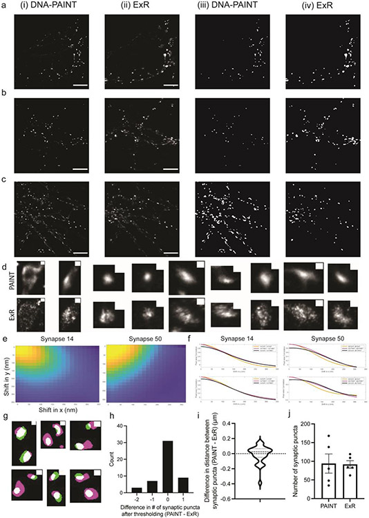
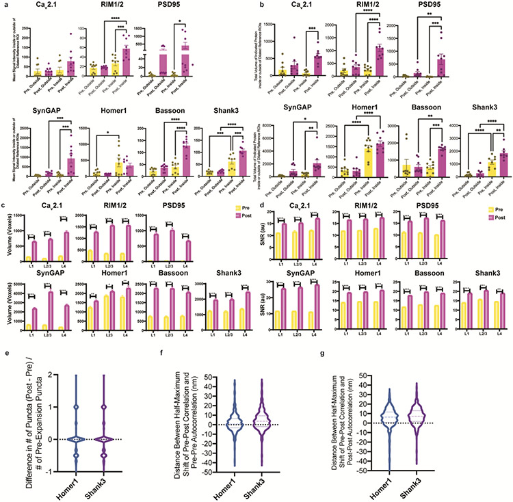
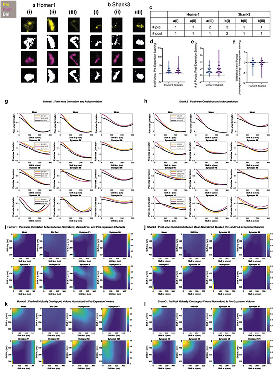
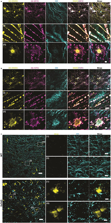
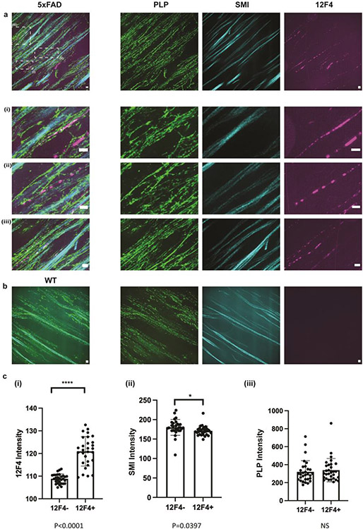
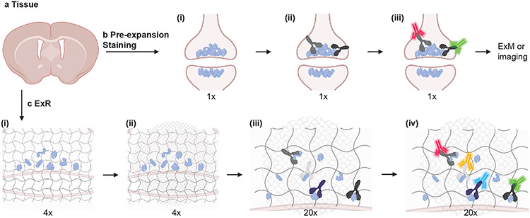
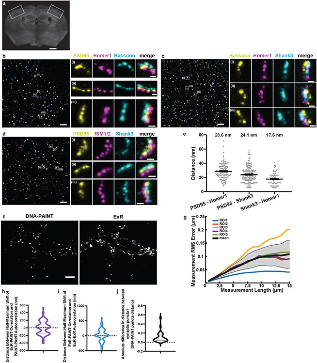
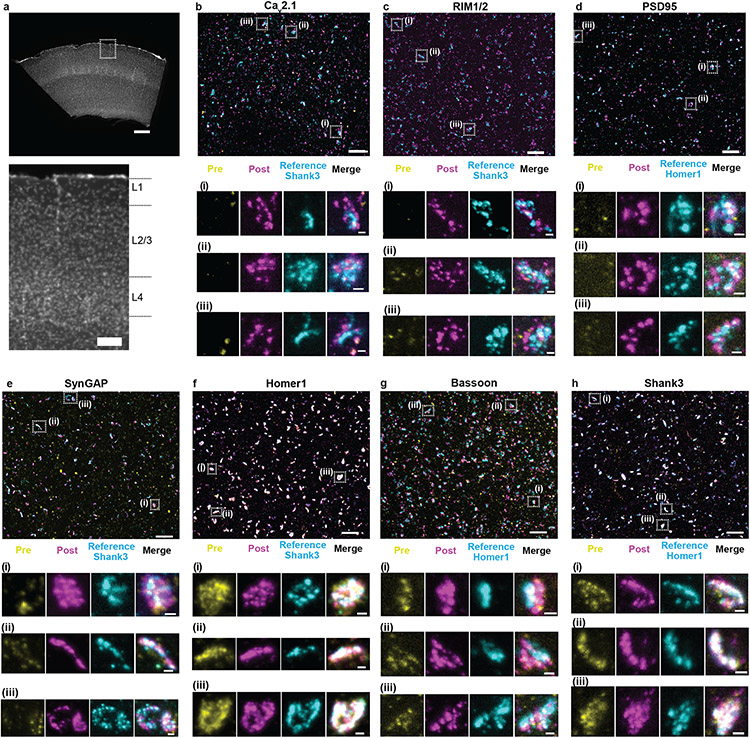
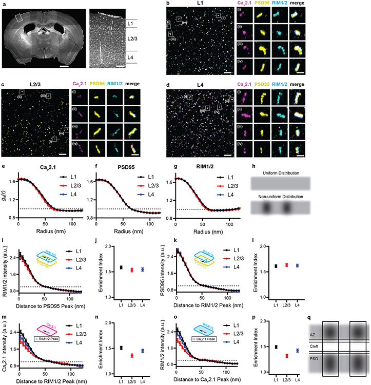
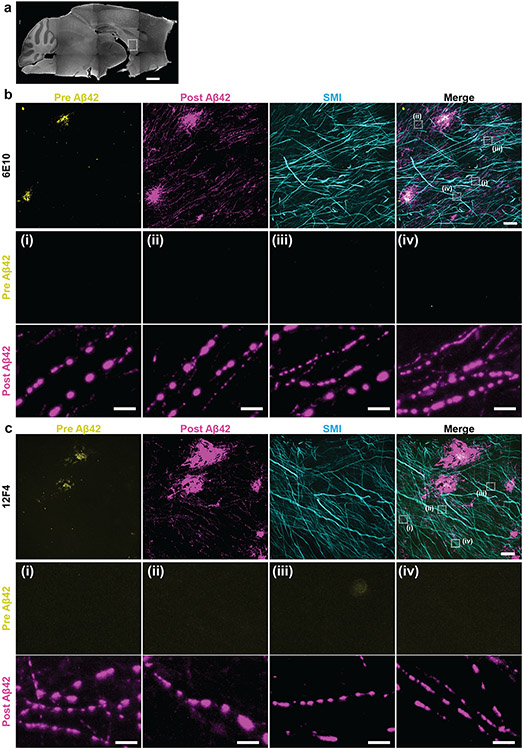
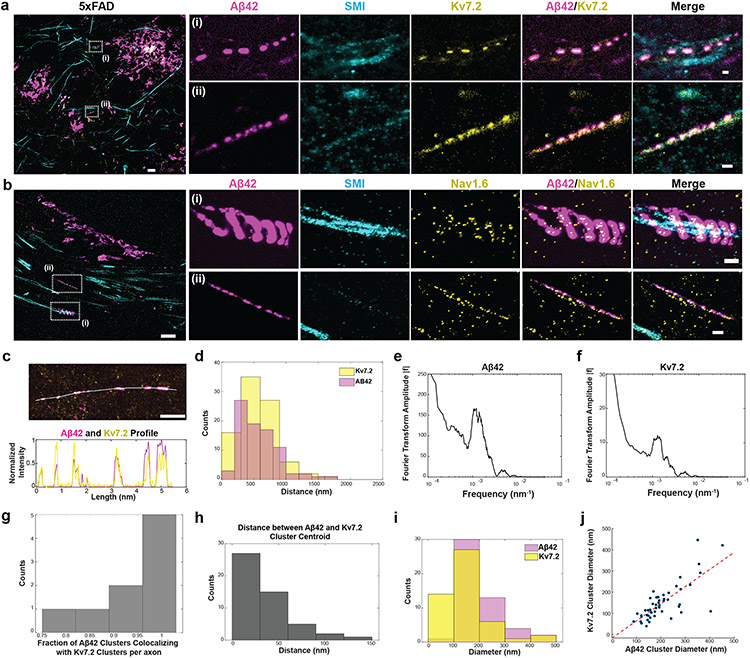
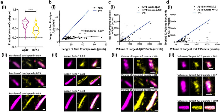
Many crowded biomolecular structures in cells and tissues are inaccessible to labelling antibodies. To understand how proteins within these structures are arranged with nanoscale precision therefore requires that these structures be decrowded before labelling. Here we show that an iterative variant of expansion microscopy (the permeation of cells and tissues by a swellable hydrogel followed by isotropic hydrogel expansion, to allow for enhanced imaging resolution with ordinary microscopes) enables the imaging of nanostructures in expanded yet otherwise intact tissues at a resolution of about 20 nm. The method, which we named 'expansion revealing' and validated with DNA-probe-based super-resolution microscopy, involves gel-anchoring reagents and the embedding, expansion and re-embedding of the sample in homogeneous swellable hydrogels. Expansion revealing enabled us to use confocal microscopy to image the alignment of pre-synaptic calcium channels with post-synaptic scaffolding proteins in intact brain circuits, and to uncover periodic amyloid nanoclusters containing ion-channel proteins in brain tissue from a mouse model of Alzheimer's disease. Expansion revealing will enable the further discovery of previously unseen nanostructures within cells and tissues.

Extended Data Fig. 1. Comparison of synaptic nanostructures imaged using DNA-PAINT and ExR in cultured neurons.

(a-c) Three representative fields of view imaged using DNA-PAINT (i) and ExR (ii) after rigid body registration to DNA-PAINT images. Scale bar = 5 μm. (iii-iv) Processed, binary versions of (i) and (ii) used to automatically count synaptic puncta number and pairwise distances. Scale bar, 5μm. (d) Representative manually-cropped matched synaptic ROIs for DNA-PAINT (top row) and ExR (bottom row), used for the distortion analysis shown in Fig. 2h,i (scale bar = 250 nm). (e) Pixel-wise correlation between min-max normalized ExR and DNA-PAINT channels as a function of shift distance in x- and y-directions for two randomly selected synaptic ROIs. (f) Pixel-wise autocorrelation between min-max normalized DNA-PAINT (PAINT-PAINT, magenta), ExR (ExR-ExR, yellow), and pixel-wise correlation between DNA-PAINT and ExR (PAINT-ExR, black) as a function of shift distance in x- and y-directions for the synaptic ROIs shown in (e). (g) Representative manually-cropped pairs of synaptic puncta used to generate the data shown in Fig. 2j and panel i. Shown is an overlay of DNA-PAINT (green) and ExR (magenta) binary masks (scale bar = 250 nm). (h) Histogram of difference in number of synaptic puncta counted after thresholding pairs of synaptic puncta. (i) Difference in radial distance between pairs of synaptic puncta, DNA-PAINT – ExR (mean = −0.008854, 95% CI [−0.05419, 0.03649]). (j) Total number of synaptic puncta for the five fields of view imaged using DNA-PAINT and ExR (two-sided paired t-test, p = 0.9271, t = 0.09735, df = 4). All data are from 5 ROIs from 3 wells of one cultured neuron batch. Shown are images from one representative experiment from two independent replicates.

Extended Data Fig. 2. Analysis of the ExR decrowding effect.

(a, b) Quantification of decrowding in a set of manually identified synapses. Statistical significance was determined using Sidak’s multiple comparisons test on two-sided t-tests following ANOVA (*P ≤ 0.05, **P ≤ 0.01, ***P < 0.001, ****P < 0.0001, here and throughout the paper, and plotted is the mean, with error bars representing standard error of the mean (SEM), here and throughout the paper). (a) Mean signal intensity inside and outside of (that is, nearby to) dilated reference ROIs for pre- and post-expansion stained manually-identified synapses (Supplementary Table 2 for numbers of technical and biological replicates)). Data points represent the mean across all synapses from a single field of view. (b) Total volume (in voxels; 1 voxel = 17.16 × 17.15 × 40, or 11,779, nm³) of signals inside and outside of dilated reference ROIs, in both cases within cropped images containing one visually identified synapse (Supplementary Fig. 3h), for pre- and post-expansion stained manually-identified synapses (Supplementary Table 2 for numbers of biological and technical replicates). Data points represent the mean across all synapses for 3 fields of view from 3 biological replicates (n = 9 fields of view total per protein). (c) Mean voxel size and (d) mean signal-to-noise (SNR) ratio of pre- and post-expansion immunostaining showing 7 proteins in somatosensory cortex regions L1, L2/3, and L4 of 3 mice. Plotted is mean and SEM. To compare the 3D voxel size and SNR of pre- and post-expansion stained synapses for each of the seven proteins, three two-sided t-tests (one for each layer) were run (n = 49-70 puncta per layer from 3 mice; Supplementary Table 2 for exact n values). Statistical significance was determined using multiple t-tests corrected using the Holm-Sidak method, with alpha = 0.05. (e) Population distribution (violin plot of density, with a dashed line at the median and dotted lines at the quartiles) of the fractional difference in the number of synaptic puncta between post- and pre-expansion staining channels for Homer1 and Shank3 (n = 480 synapses from 3 mice). (f) Population distribution of the difference in distance (in nm) between the shift at which the correlation is half maximal half-maximal shift for pre-pre autocorrelation and post-pre correlation (calculated pixel-wise between intensity values normalized to the minimum and maximum of the image, see Methods) for x-, y-, and z-directions (x- and y-directions being transverse, z-direction being axial) for Homer1 and Shank3 (n = 458 synapses, 3 directions each, from 3 mice). (g) Same as (f), for post-post autocorrelation and pre-post correlation.

Extended Data Fig. 3. Analysis of the distortion caused by post-expansion staining, as compared to classical pre-expansion staining.

(a-b) Representative background-subtracted and binary images of Homer1 (a) and Shank3 (b) in pre- and post-expansion staining channels (top row (yellow): pre-expansion channel, second row (black/white): binary pre-expansion channel, third row (magenta): post-expansion channel, bottom row (black/white): binary post-expansion channel). (c) Number of synaptic puncta for pre- and post-expansion staining channels, after filtration, for the images in (a-b). (d) Population distribution (violin plot of density, with a dashed line at the median and dotted lines at the quartiles) of the number of synaptic puncta in the pre-expansion staining channel for Homer1 and Shank3 (see Supplementary Table 5 for statistics for this figure). (e) Population distribution of the number of synaptic puncta in the post-expansion staining channel for Homer1 and Shank3. (f) Difference in the number of synaptic puncta between post- and pre-expansion staining channels normalized to the number of synaptic puncta in the pre-expansion staining channel. (g-h) Pixel-wise autocorrelation between pre-expansion (pre-pre, yellow), post-expansion (post-post, magenta), and pixel-wise correlation between pre- and post-expansion (pre-post, black) as a function of shift distance in x- (left column), y- (middle column), and z- (right column) directions for Homer1 (g) and Shank3 (h). The mean across all synapses is shown in the top row, and representative synapses are shown in the second through fourth rows. These values were used to calculate the linearized error measure shown in Extended Data Fig. 2f, g. (i-j) Pixel-wise correlation between mean-normalized, masked pre- and post-expansion channels as a function of shift distance in x- and y-directions (z = 1) for Homer1 (i) and Shank3 (j). The mean across all synapses is shown in the top left, standard deviation across all synapses shown in second from the top left, and representative synapses are shown in the remaining plots. (k-l) Mutually overlapped volume between pre- and post-expansion stained synaptic puncta, normalized to total puncta volume in the pre-expansion staining channel, as a function of shift distance in x- and y-directions (z = 1) for Homer1 (k) and Shank3 (l). The mean across all synapses is shown in the top left, standard deviation across all synapses shown in second from the top left, and representative synapses are shown in the remaining plots. Analysis was conducted on 480 (before exclusion based on size) synapses for Shank3 and Homer1 from 3 mice (see Supplementary Table 5 for exact numbers).

Extended Data Fig. 4. ExR and unexpanded tissue confocal images showing immunolabeling of Aβ42.

ExR confocal images (single z-slices) showing immunolabeling of Aβ42 with two different monoclonal antibodies (a) D54D2 + 6E10 and (b) D54D2 + 12F4 with SMI co-staining in the fornix of 5xFAD mouse (n = 3 fields of view of 2 slices from 2 mice). Scale bar, 10 μm (top row), 1 μm (i, ii panels). (c) Unexpanded tissue confocal image, a single z-slice, showing pre-expansion Aβ42 (yellow) and SMI (cyan) staining in the fornix of WT (upper panel) and 5xFAD mice (lower panel) (n = 3 fields of view of 1 slice from 1 mouse per WT and 5xFAD, respectively). Scale bar, 30 μm (left panel) and 6 μm (panels i, ii)).

Extended Data Fig. 5. ExR confocal images showing immunolabeling of PLP, SMI, and 12F4 in 5xFAD and WT fornix.

ExR reveals relative localization of Aβ42 peptide and myelin in the fornix of Alzheimer’s model 5xFAD and WT mice (n = 2 fields of view of 1 slice from 2 mice per WT and 5xFAD, respectively). (a) ExR confocal image (max intensity projections, 900–1000 nm thickness) showing post-expansion Aβ42 (magenta), SMI (cyan) and PLP (green) staining in the fornix of 5xFAD mice. Leftmost panel, merged low-magnification image; right images show individual channels. Insets (i-iii) show close-up views of the boxed regions highlighted in the upper left image. (b) ExR confocal image (max intensity projections, 1.72 μm thickness) showing post-expansion Aβ42 (magenta), SMI (cyan) and PLP (green) staining in the fornix of wild-type mice. Leftmost panel, merged image. All images were subtracted background using Fiji’s Rolling Ball algorithm with radius 50 pixels, and adjusted with auto-contrast. Scale bar = 500 nm. (c) Comparison of 12F4, SMI, and PLP intensity levels along axons in 5xFAD fornix with and without 12F4. To analyze axonal amyloid beta deposition with myelination and SMI intensity, we measure the (i) 12F4, (ii) SMI and (iii) PLP intensity levels along 10 axons with (12F4+) and without 12F4 (12F4−) from the same field of view (n = 3 fields of view of 2 slices from 2 5xFAD). All images were subtracted background with 50 pixels, and adjusted with auto-contrast for analysis by ImageJ. On each axon, three lines were drawn cross-sectionally across each axon in Image J and averaged intensity levels of PLP, 12F4 and SMI from different channels were measured respectively along these lines. For 12F4 + axons, each line was drawn across the centroid of amyloid beta deposition. For 12F4− axons, lines were positioned randomly along the axon. We then compared PLP, 12F4 and SMI312 intensity levels between 12F4 + and 12F4− axons. Plotted is the mean, with error bars representing standard error of the mean (SEM). Two-sided paired t-test, (i) ****p < 0.0001, t = 6.112, df = 18, (ii) p = 0.0595, t = 2.012, df = 18, (iii) p = 0.6580, t = 0.4502, df = 18.

Fig. 1 ∣. Expansion Revealing (ExR), a technology for decrowding of proteins through isotropic protein separation.

(a) Coronal section of mouse brain before staining or expansion. (b) Conventional antibody staining may not detect crowded biomolecules, shown here in pre- and post-synaptic terminals of cortical neurons. (b i) Crowded biomolecules before antibody staining. (b ii) Primary antibody (Y-shaped proteins) staining in non-expanded tissue. Antibodies cannot access interior biomolecules, or masked epitopes of exterior biomolecules. (b iii) Secondary antibody (fluorescent green and red Y-shaped proteins) staining in non-expanded tissue. After staining, tissue can be imaged or expanded using earlier ExM protocols, but inaccessible biomolecules will not be detected. (c) Post-expansion antibody staining with ExR. (c i) Anchoring and first gelation step. Specimens are labelled with gel-anchoring reagents to retain endogenous proteins, with acrylamide included during fixation to serve as a polymer-incorporatable anchor, as in refs^,. Subsequently, the specimen is embedded in a swellable hydrogel that permeates densely throughout the sample (gray wavy lines), mechanically homogenized via detergent treatment and heat treatment, and expanded in water. (c ii) Re-embedding and second swellable gel formation gelation. The fully expanded first gel (expanded 4x in linear extent) is re-embedded in a charge-neutral gel (not shown), followed by the formation of a second swellable hydrogel (light grey wavy lines). (c iii) 20x expansion and primary antibody staining. The specimen is expanded by another factor of 4x, for a total expansion factor of ~20x, via the addition of water, then incubated with conventional primary antibodies. Because expansion has decrowded the biomolecules, conventional antibodies can now access interior biomolecules and additional epitopes of exterior molecules. (c iv) Post-expansion staining with conventional fluorescent secondary antibodies (fluorescent blue and yellow Y-shaped proteins, in addition to the aforementioned red and green ones) to visualize decrowded biomolecules. Schematic created with BioRender.com.

Fig. 2. Validation of ExR using synapses and comparison with DNA-PAINT.

(a) Low-magnification widefield image of a mouse brain slice stained with DAPI, with box highlighting the somatosensory cortex used in subsequent figures for synapse staining (Scale bar, 500 μm), and (b-d) confocal images (max intensity projections) of representative fields of view (cortical L2/3) and specific synapses after ExR expansion and subsequent immunostaining using antibodies against (b) PSD95, Homer1, Bassoon; (c) Bassoon, Homer1, Shank3; and (d) PSD95, RIM1/2, Shank3. Scale bar, 1 μm, left image; 100 nm, right images; in biological units, i.e. the physical size divided by the expansion factor, throughout the paper unless otherwise indicated. Shown are images from one representative experiment from two independent replicates. (e) Measured distance between centroids of protein densities of PSD95 and Homer1, PSD95 and Shank3, and Shank3 and Homer1, in synapses such as those in panels b-d. The mean distance (again, in biological units) between PSD95 and Homer1 is 28.6 nm (n = 126 synapses from 3 slices from 1 mouse), between PSD95 and Shank3 is 24.1 nm (n=172 synapses from 3 slices from 1 mouse), and between Shank3 and Homer1 is 17.6 nm (n=70 synapses from 3 slices from 1 mouse). Plotted is mean +/− standard error; individual grey dots represent the measured distance for individual synapses. (f) A pre-expansion DNA-PAINT image (left) and a registered confocal ExR image (max intensity projection, right) of the same field of cultured neurons after immunostaining with antibodies against Synapsin 1. Scale bar, 4 μm. Shown are images from one representative experiment from two independent replicates. (h) Estimated population distribution (violin plot of density, with a dashed line at the median and dotted lines at the quartiles) of the shift (in nm) at which the correlation is half-maximal for PAINT-PAINT autocorrelation and ExR-PAINT correlation (calculated pixel-wise between intensity values normalized to the minimum and maximum of the image, see Methods; see Supplementary Table 1 for statistics. n = 101 synaptic ROIs from 5 fields of view from 3 wells of cultured neurons from 1 culture batch). (i) Same as (h), for ExR-ExR autocorrelation vs. ExR-PAINT correlation. (j) Estimated population distribution (violin plot of density, with a dashed line at the median and dotted lines at the quartiles) of the normalized absolute difference in radial distance between neighbouring synaptic puncta centroids (Absolute value of PAINT-ExR, normalized to PAINT distance; see Supplementary Table 1 for statistics. n = 27 cropped synaptic pair ROIs from 5 fields of view of 30 μm x 30 μm each, 1 culture batch). (g) Root mean square error vs. measurement length (in biological units), calculated via a non-rigid registration algorithm of DNA-PAINT vs. ExR-processed cultured neurons (n=5 fields of view from 3 wells from 1 culture batch). Black line, mean; gray shading, standard deviation.

Fig. 3 ∣. Validation of ExR enhancement and effective resolution in synapses of mouse cortex.

(a) Low-magnification widefield image of a mouse brain slice with DAPI staining showing somatosensory cortex (top) and zoomed-in image (bottom) of boxed region containing L1, L2/3, and L4, which are imaged and analyzed after expansion further in panels b-h. (Scale bar, 300 μm (top) and 100 μm (bottom)). (b-h) Confocal images of (max intensity projections) of specimen after immunostaining with antibodies against Cav2.1 (Ca²⁺ channel P/Q-type) (b), RIM1/2 (c), PSD95 (d), SynGAP (e), Homer1 (f), Bassoon (g), and Shank3 (h), in somatosensory cortex L2/3. For pre-expansion staining, primary and secondary antibodies were stained before expansion, the stained secondary antibodies anchored to the gel, and finally fluorescent tertiary antibodies applied after expansion to enable visualization of pre-expansion staining. For post-expansion staining, the same primary and secondary antibodies were applied after ExR. Antibodies against Shank3 (b, c, e, f) or Homer1 (d, g, h) were applied post-expansion as a reference channel. Confocal images of cortex L2/3 (top) show merged images of pre- and post-expansion staining, and the reference channel. Zoomed-in images of three regions boxed in the top image (i-iii, bottom) show separate channels of pre-expansion staining (yellow), post-expansion staining (magenta), reference staining (cyan), and merged channel. (Scale bar, 1.5 μm (upper panel); 150 nm (bottom panel of i-iii).) Shown are images from one representative experiment from two independent replicates.

Fig. 4 ∣. ExR reveals how calcium channel distributions participate in transsynaptic nanoarchitecture.

(a) Low-magnification widefield image of DAPI stained mouse brain slice (left) and zoomed in view (right) of the boxed region showing layers 1-4 of the cortex. (Scale bar = 1000 μm (left panel of whole brain) and 100 μm (right panel of the layers 1-4). (b-d) show confocal images (max intensity projections) of layers 1, 2/3 and 4 respectively, after performing ExR and immunostaining with antibodies against Cav2.1 (calcium channel) (magenta), PSD95 (yellow) and RIM1/2 (cyan). In each of (b), (c) and (d), low magnification images are shown on the left while zoomed-in images of four regions, i-iv are shown on the right with separated channels for each antibody along with the merged image. (Scale bar = 1 μm (left panel) and 100 nm (right panels labelled i-iv)). Shown are images from one representative experiment from two independent replicates. (e-g) show the autocorrelation analysis for Cav2.1, PSD95 and RIM1/2 respectively for different layers. (h) shows schematic illustration of protein distribution based on interpretation of autocorrelation results in (e-g). A uniform distribution (h, top) would be predicted if g_a(r) = 1 at all radii (dotted lines in e-g), whereas a non-uniform distribution with one or more regions of high local intensity (h, bottom) would be predicted if g_a(r) was greater than 1 at short radii and decayed as the radius is increased. (i), (k), (m) and (o) show the enrichment analysis that calculates the average molecular density for RIM1/2 to the PSD95 peak, PSD95 to the RIM1/2 peak, Cav2.1 to the RIM1/2 peak and RIM1/2 to the Cav2.1 peak respectively while (j), (l), (n) and (p) show the corresponding mean enrichment indexes respectively (see Methods for exact n - values). Error bars indicate SEM. (q) shows schematic illustration of protein distribution based on interpretation of enrichment analysis results in (i-p). Enrichment values above 1 represent regions of high local intensity in the measured channel, so the enrichment profiles in (i), (k), (m) and (o) suggest the peak of the reference channel closely aligns with regions of high intensity in the measured channel for each of the four comparisons. Therefore, this suggests that enriched regions of any two proteins (RIM1/2, PSD95 and Cav2.1) are aligned in nanoscale precision with each other. Calcium channels located close to vesicle fusion sites (dictated by RIM1/2) may enhance the calcium-sensitivity of fusion. Additionally, postsynaptic receptors may be exposed to higher, faster peaks of neurotransmitter concentration when vesicle release sites are located directly opposite receptor nanoclusters (PSD95 being a receptor-anchoring protein). (AZ: active zone, PSD: postsynaptic density).

Fig. 5 ∣. ExR reveals periodic nanoclusters of Aβ42 peptide in the fornix of Alzheimer’s model 5xFAD mice.

(a) Epifluorescence image showing a sagittal section of a 5xFAD mouse brain with the fornix highlighted. (Scale bar, 1000 μm) (b-c) ExR confocal Images (max intensity projections) showing immunolabelling against Aβ42 peptide with two different monoclonal antibodies 6E10 (b) and 12F4 (c). From left to right: pre-expansion immunolabelling of Aβ42 (yellow), post-expansion labelling (magenta) of Aβ42, post-expansion SMI (neurofilament protein), and merged pre- and post-expansion staining of Aβ42 with post-expansion staining of SMI. Insets (i-iv) show regions of interest highlighted in the merged images in the fourth column; top panels, pre-expansion Aβ42 labelling; middle panels, post-expansion Aβ42 labelling; bottom panels, post-expansion SMI labelling. Post-ExR staining reveals periodic nanostructures of β-amyloid, whereas pre-expansion staining can detect only large plaque centers. (Scale bar = 10 μm (upper panel images); 1 μm (bottom panels, i-iv))

Fig. 6 ∣. ExR reveals co-localized clusters of Aβ42 peptide with potassium and sodium ion channels in the fornix of Alzheimer’s model 5xFAD mice.

(a-b) ExR confocal image (max intensity projections) showing post-expansion (a) Aβ42 (magenta), SMI (cyan) and Kv7.2 (yellow) staining, and (b) Aβ42 (magenta), SMI (cyan) and Nav1.6 (yellow) staining in the fornix of a 5xFAD mouse. Leftmost panel, merged low magnification image. (Scale bar = 4 μm); insets (i-ii) show close-up views of the boxed regions in the leftmost image for (A) Aβ42, SMI, Kv7.2, Aβ42-Kv7.2 merged and Aβ42-Kv7.2-SMI merged respectively, and (b) Aβ42, SMI, Nav1.6, Aβ42-Nav1.6 merged and Aβ42-Nav1.6-SMI merged respectively (scale bar = 400 nm; n = 5 fields of view from 2 slices from 2 mice). (c) ExR confocal image (max intensity projections) showing Aβ42 (magenta) and Kv7.2 (yellow) clusters in a 5xFAD mouse (top) with the indicated cross-section profile shown (bottom). (Scale bar = 1 μm). Shown are images from one representative experiment from four independent replicates. (d) Histograms showing distances between adjacent Aβ42 (magenta) and Kv7.2 (yellow) clusters in 5xFAD mice along imaged segments of axons (n=97 Aβ42 clusters, 92 Kv7.2 clusters from 9 axonal segments from 2 mice). (e-f) Fourier transformed plots of Aβ42 (e) and Kv7.2 (f) showing the same peak position (from the same data set as (d)). (g) Histogram showing the fraction of Aβ42 clusters colocalizing with Kv7.2 clusters along individual segments of axons (n=50 cluster pairs from 9 axonal segments from 2 mice). (h) Histogram showing the distance between the centroids of colocalized Aβ42 and Kv7.2 clusters (same data set as (d)). (i) Histograms showing the diameters of Aβ42 clusters (magenta) and Kv7.2 clusters (yellow) (n=50 cluster pairs from 9 axonal segments from 2 mice). (j) Scatter plot showing the diameters of colocalized Aβ42 and Kv7.2 clusters.

Fig. 7 ∣. Analysis of Aβ42 peptide and potassium ion channels nanoclusters in shapes and their relationships.

(a)(i) Fraction of total Aβ42 and Kv7.2 puncta volume overlapped with one another in cropped Aβ42 clusters (n = 55 clusters from 2 5xFAD mice; p < 0.0001, two-sided pairwise t-test). ****P < 0.0001. (a)(ii) Representative images illustrating the difference in the proportion of mutually overlapped volume between Aβ42 and Kv7.2 as a fraction of total Aβ42 or Kv7.2 volume (scale bar = 100nm). (b)(i) Length of the second principal axis of the ellipsoid that has the same normalized second central moments as the largest Aβ42 punctum in an ROI, vs. the length of the first principal axis of this ellipsoid (in pixels, 1 pixel = 11.44 nm in x- and y-directions (transverse) and 26.67nm in the z-direction (axial); black points represent individual manually cropped ROIs; slope of best-fit line from simple linear regression = 0.05883, p = 0.0020, F = 10.59, df = 53). Compare to the line y = x (blue). (b)(ii) Representative images illustrating the oblong shape of Aβ42 puncta, for three first principal axis lengths: shorter (top row), medium (middle row) and longer (bottom row). While the length of the first principal axis varies significantly between these examples, the length of the second principal axis remains similar between the three clusters. (c)(i) Total volume (in voxels, 1 voxel = 11.44x11.44x26.67 or 3,490 nm3) of Kv7.2 puncta overlapped/inside (black, R² = 0.980, p < 0.0001) and outside (gray, R² = 0.0582, p = 0.0979) Aβ42 puncta, as a function of the volume of the largest Aβ42 puncta within an ROI, compared to the line y = x (blue). (c)(ii) Representative images illustrating that the volume of Kv7.2 outside of Aβ42 is relatively constant as Aβ42 puncta size increases. As in (b)(ii), the three clusters shown are ordered by increasing size. (d) The converse of (c): total volume of Aβ42 puncta overlapped/inside (black, R² = 0.6531, p < 0.0001) and outside (gray, R² = 0.1876, p = 0.0010) of Kv7.2 puncta, as a function of the volume of the largest Kv7.2 puncta within an ROI, compared to the line y = x (blue). (d)(ii). Representative images illustrating that the volume of Aβ42 outside of Kv7.2 is smaller than the volume of Aβ42 co-localized with Kv7.2, and both values are positively correlated with the volume of the largest Kv7.2 puncta. Scale bar of (a-d ii) = 100 nm. Shown are images from one representative experiment from four independent replicates.

References

1. Sydor AM, Czymmek KJ, Puchner EM & Mennella V Super-Resolution Microscopy: From Single Molecules to Supramolecular Assemblies. Trends in Cell Biology vol. 25 730–748 (2015). - PubMed
1. Wassie AT, Zhao Y & Boyden ES Expansion microscopy: principles and uses in biological research. Nature Methods vol. 16 33–41 (2019). - PMC - PubMed
1. Chen F, Tillberg PW & Boyden ES Expansion microscopy. Science 347, 543–548 (2015). - PMC - PubMed
1. Chang JB et al. Iterative expansion microscopy. Nat. Methods 14, 593–599 (2017). - PMC - PubMed
1. Chen F et al. Nanoscale imaging of RNA with expansion microscopy. Nat. Methods 13, 679–684 (2016). - PMC - PubMed
Publication types
LinkOut - more resources