. 2022 Sep;25(9):1124-1128.
doi: 10.1038/s41593-022-01152-z. Epub 2022 Aug 30.

Fiber photometry in striatum reflects primarily nonsomatic changes in calcium

Affiliations

Fiber photometry in striatum reflects primarily nonsomatic changes in calcium

Alex A Legaria et al. Nat Neurosci. 2022 Sep.

Abstract

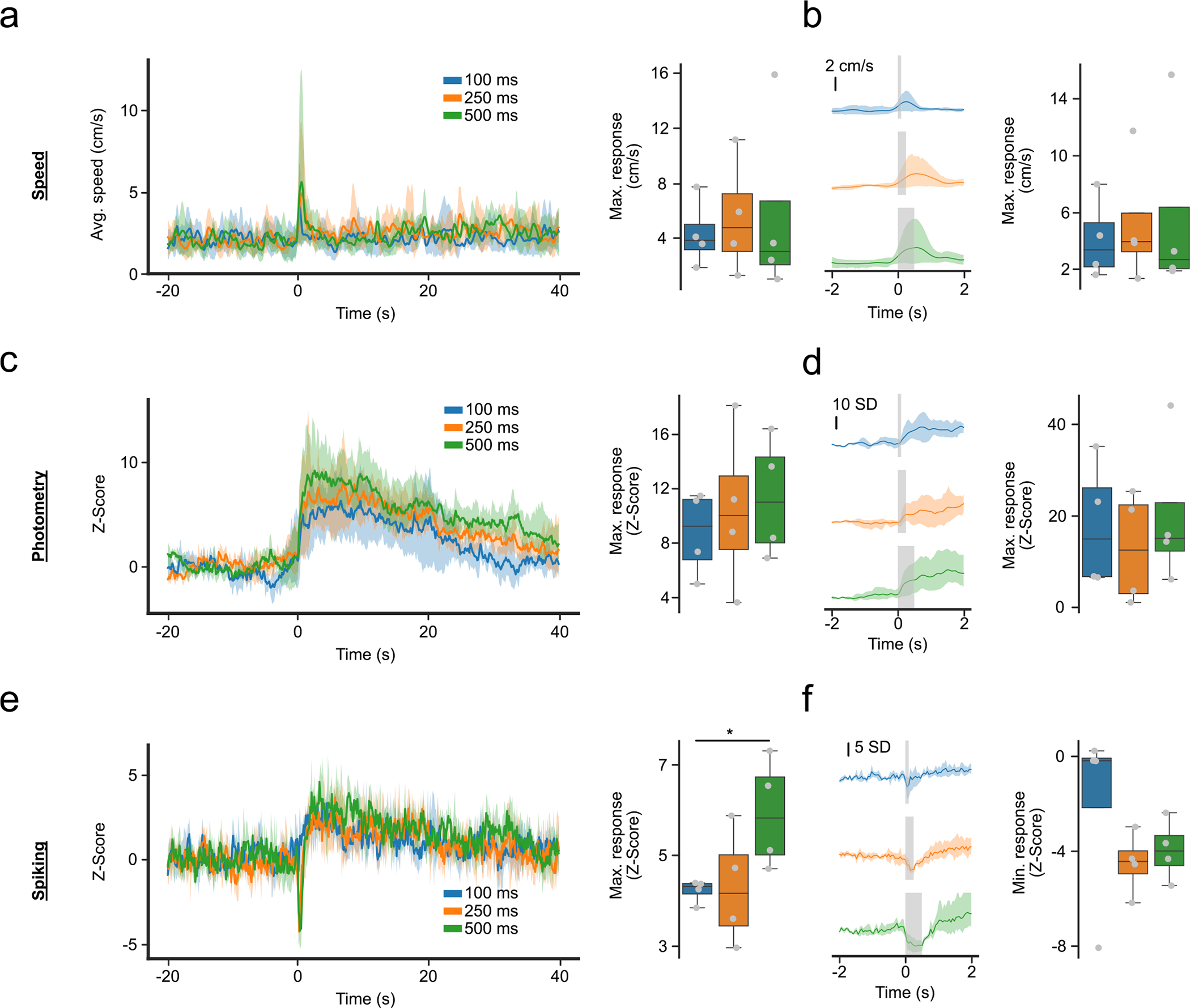
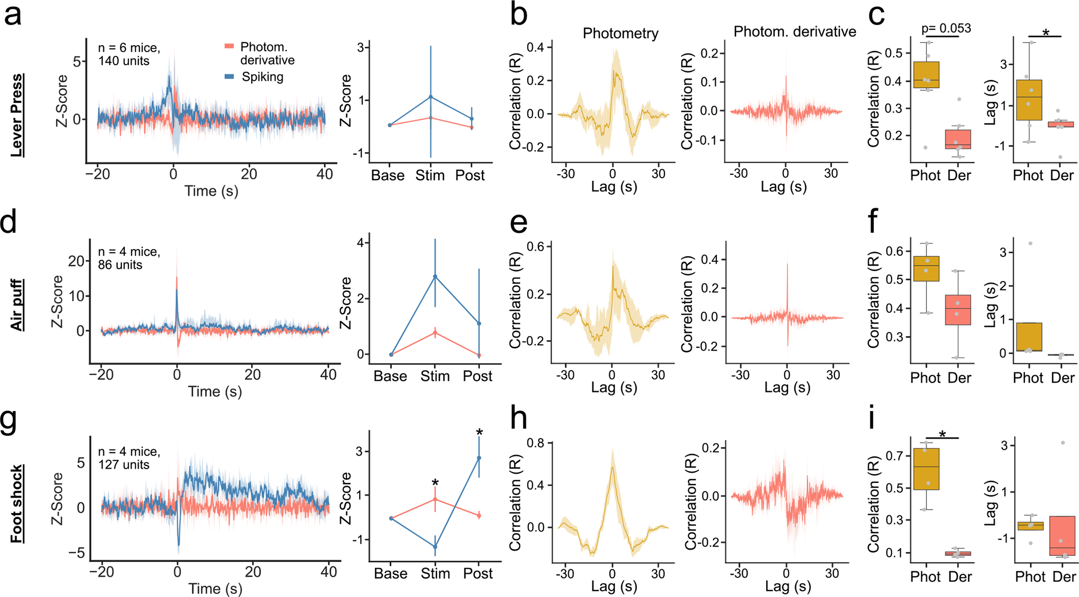
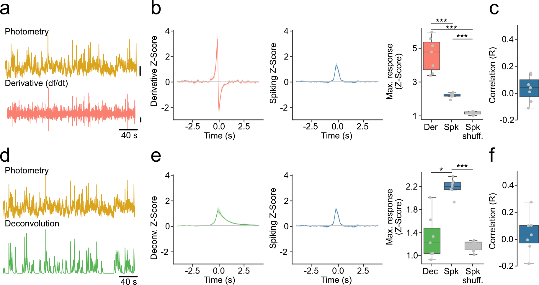
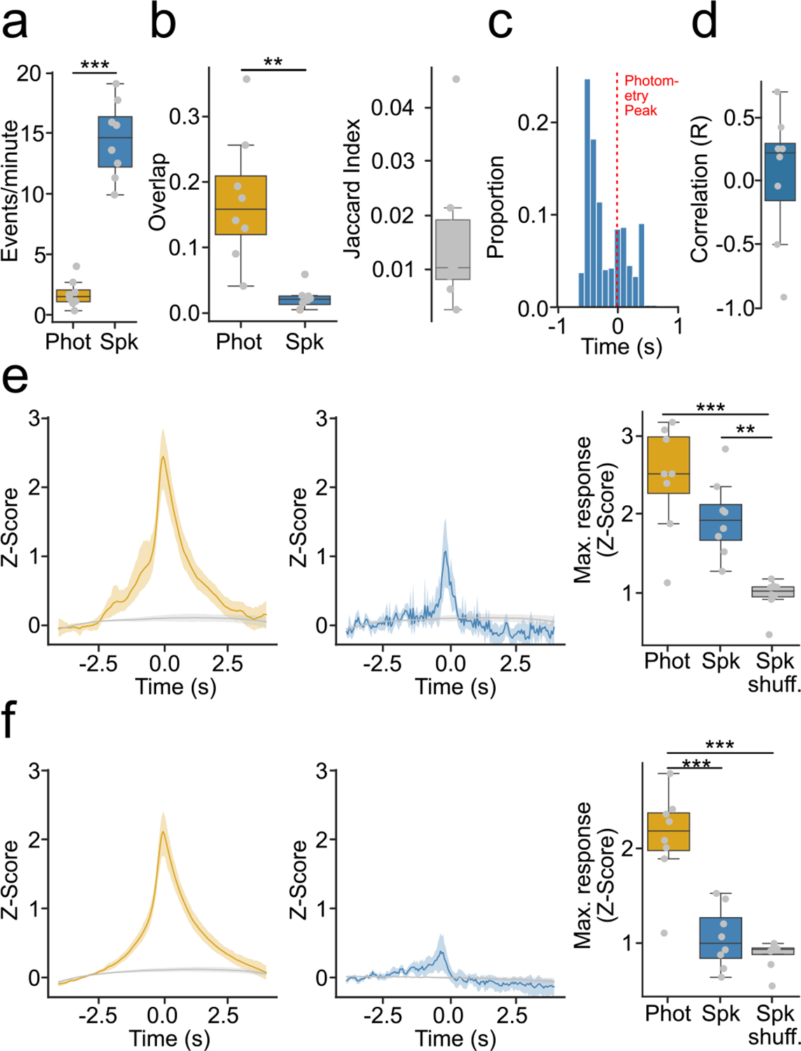
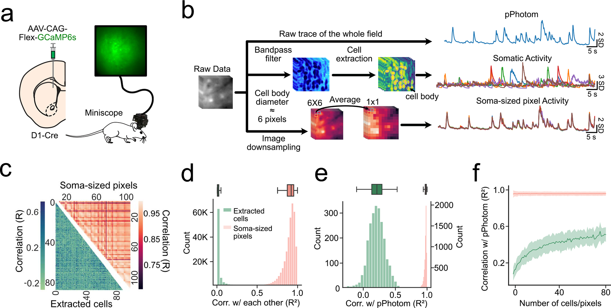
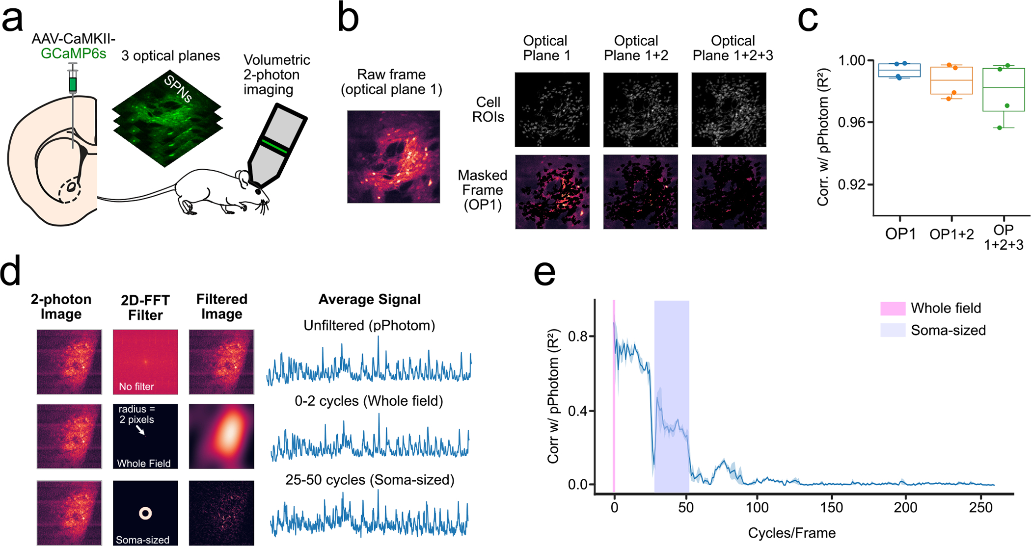
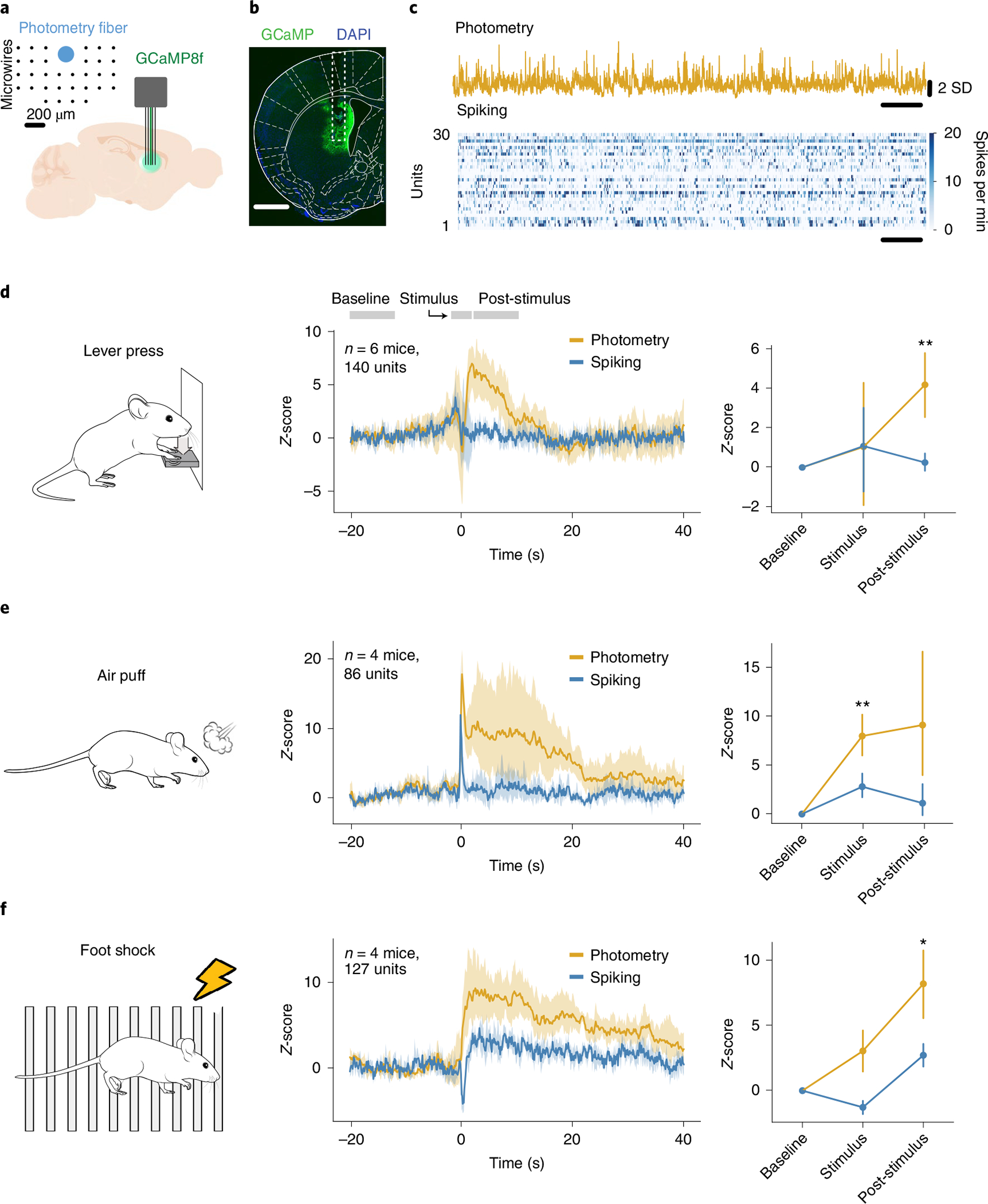
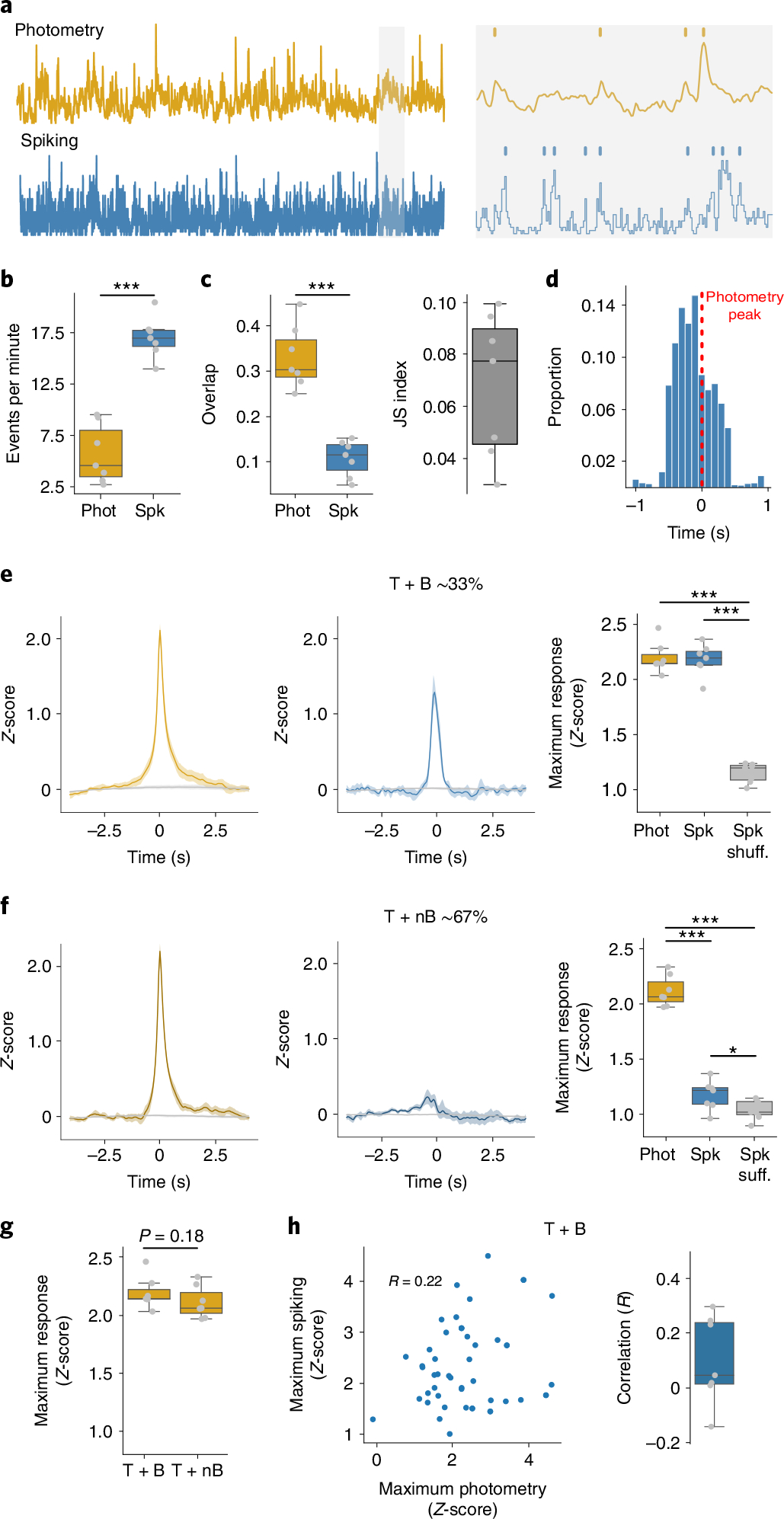
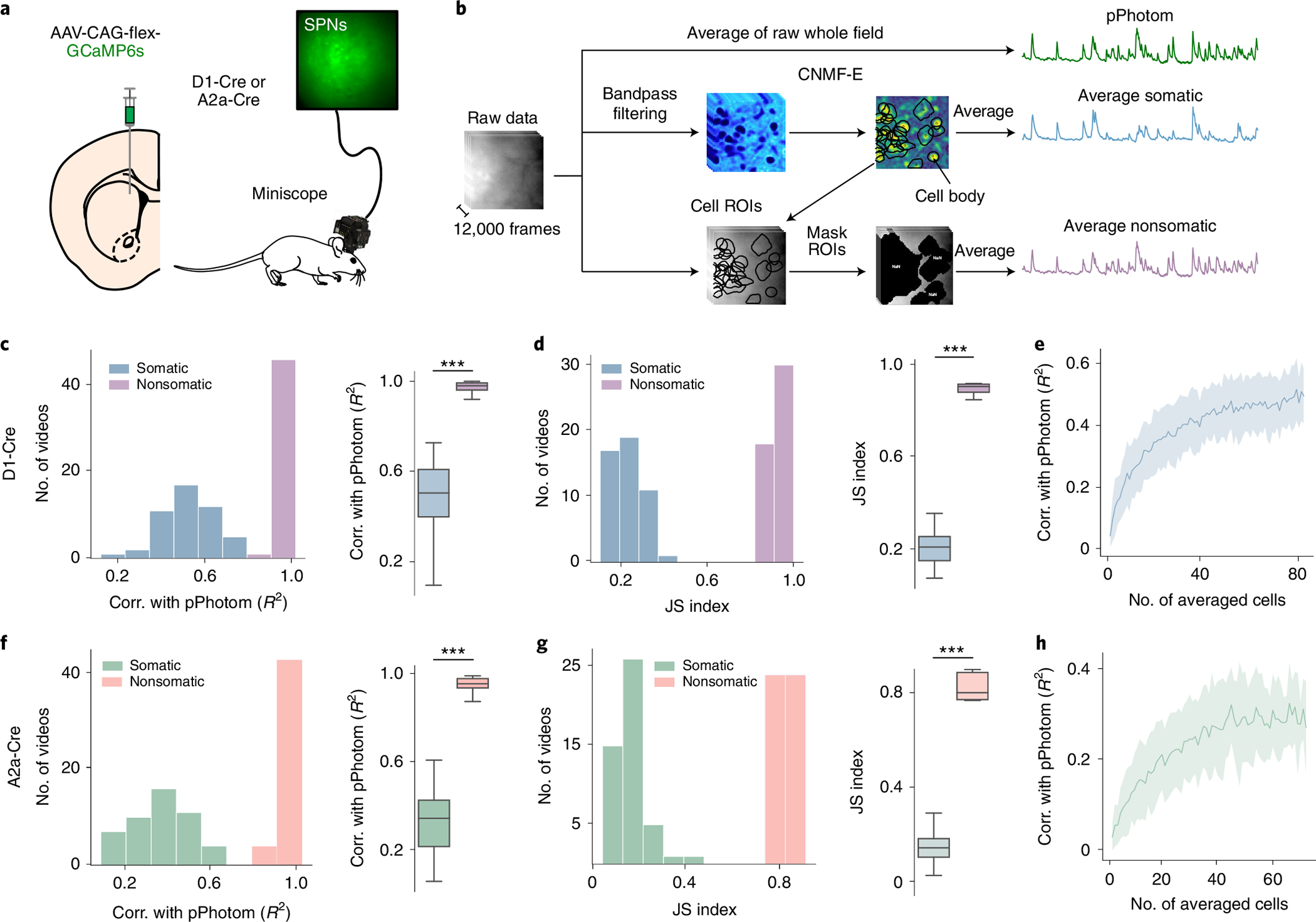
Fiber photometry enables recording of population neuronal calcium dynamics in awake mice. While the popularity of fiber photometry has grown in recent years, it remains unclear whether photometry reflects changes in action potential firing (that is, 'spiking') or other changes in neuronal calcium. In microscope-based calcium imaging, optical and analytical approaches can help differentiate somatic from neuropil calcium. However, these approaches cannot be readily applied to fiber photometry. As such, it remains unclear whether the fiber photometry signal reflects changes in somatic calcium, changes in nonsomatic calcium or a combination of the two. Here, using simultaneous in vivo extracellular electrophysiology and fiber photometry, along with in vivo endoscopic one-photon and two-photon calcium imaging, we determined that the striatal fiber photometry does not reflect spiking-related changes in calcium and instead primarily reflects nonsomatic changes in calcium.


Conflict of interest statement

Competing interests

The authors declare no competing interests.

Figures

Extended Data Fig. 1 |
Extended Data Fig. 1 |. Photometry, and spiking activity, and locomotor activity reflect distinct responses around foot shocks.
(a) Motor response around 0.7 mA foot shocks of different length. (Left) Average response from −20 to 40 seconds. (Right) Maximum response from 0 to 5 seconds, time-locked to foot shock (F-Value = 0.64, p-value = 0.558). (b) Close-up of (a), showing motor response in a short time-interval around foot shock. (Left) Average response from −2 to 2 seconds. (Right) Maximum response from 0 to 1 second, excluding the stimulus time (F-value = 0.61, p-value = 0.572). (c) Same as (a) but for the photometry response. (Right) F-value = 0.93, p-value = 0.445. (d) Same as (b) but for photometry response. (Right) F-value = 1.89, p-value = 0.231. (e) Same as (a,c) for spiking activity. (Right) F-value = 8.57, p-value = 0.017 (f) Same as (b,d) but for spiking activity and showing the minimum response instead of maximum. (Right) F-value = 1.38, p-value = 0.321. For quantification, we ran repeated measures ANOVAs with post-hoc two-tailed paired t-tests with bonferroni corrections (n = 4 mice). * denotes p < 0.05 after correction. Shaded regions represent 95% confidence intervals. Box plots central value denotes the median, box bounds denote upper and lower quartiles and whiskers denote ±1.5 interquartile range.
Extended Data Fig. 2 |
Extended Data Fig. 2 |. The time derivative of photometry (derivative) and spiking activity show distinct responses to behavioral events.
(a) Derivative and population spiking response around lever press (n = 6 mice). (Left) Average response. (Right) Average response in baseline, stimulus and post-stimulus intervals (Signal~Interval F-Value = 0.33, p-value = 0.724). (b) Cross-correlations between the response of the population spiking and photometry (Left) and derivative (Right). (c) (Left) Maximum correlation between photometry and spiking (yellow), and derivative and spiking (pink); p-value = 0.053. (Right) Latency to maximum correlation (n = 6 mice); p-value = 0.027. (d–f) Same as (a-c) for air puff stimulus (n = 4 mice). (d, Right) Signal~Interval F-Value = 4.1, p-value = 0.075. (g-i) Same as (a-c, d-f) for foot shock stimulus (n = 5 mice); i-right: p-value = 0.013. (g, right) Signal~Interval F-Value = 22.22, p-value = 0.002. For quantification of (a,d,f), we ran a repeated measures ANOVA, with post-hoc two-tailed paired t-test with bonferroni corrections. For quantification of (c,f,h), we ran 2-tailed paired t-tests. * denotes p < 0.05. Line plots show mean±95% confidence interval. error bars in (a,d,g right) denote standard deviation. Box plots central value denotes the median, box bounds denote upper and lower quartiles and whiskers denote ±1.5 interquartile range.
Extended Data Fig. 3 |
Extended Data Fig. 3 |. The time derivative and deconvolution of fiber photometry spiking activity.
(a) Example photometry trace (top) and its derivative (bottom). Vertical lines represent 2 standard deviations. (b) Derivative and spiking response around photometry transients overlapping with a spiking burst (T + B). (Left) Average derivative response. (Middle) Average population spiking response. (Right) Maximum response (n = 7 mice, F-stat = 60.80, p-value = 1 × 10⁻⁵). (c) Correlations between maximum derivative (Der) and population spiking (Spk) response around T + B. (d) Example photometry trace (top) and its respective deconvolution (bottom). Vertical lines represent 2 standard deviations. (e) Same as (b) but for deconvolution instead of derivative (n = 7 mice, F-stat = 37.74, p-value = 1 × 10⁻⁵). (f) Correlations between maximum deconvolution (Dec) and population spiking (Spk) response around T + B. Shaded regions represent 95% confidence intervals. Box plots central value denotes the median, box bounds denote upper and lower quartiles and whiskers denote ±1.5 interquartile range. For quantification of (b,e right), we used a repeated measures ANOVA with post-hoc two-tailed paired t-tests with Bonferroni corrections. * denotes p < 0.05; *** denotes p < 0.001 after corrections.
Extended Data Fig. 4 |
Extended Data Fig. 4 |. GcaMP6s fiber photometry reflects only a small proportion of spontaneous changes in spiking activity.
(a) Frequency of identified events in photometry or spiking (n = 8 mice, p-value = 1.75 × 10⁻⁵). (b) Similarity of photometry and spiking events (n = 8 mice). (Left) Proportion of overlap between photometry and spiking events (p-value = 2.36 × 10⁻⁴). (Right) Jaccard similarity. (c) Time course of maximum spiking activity around transients that overlapped with bursts (T + B). (d) Average correlations between photometry and spiking responses atound T + B. (e) Photometry and spiking response around T + B or shuffled timestamps. (Left) Average photometry response T + B (yellow) or shuffled timestamps (gray). (Middle) Average spiking response around T + B (blue) or shuffled timestamps (gray). (Right) Average maximum photometry/spiking response (n = 8 mice, F-value = 20.68, p-value = 1 × 10⁻⁵). (f) Same as (e) but for transients that did not overlap with bursts (T + nB) (Right) (n = 8 mice, F-value = 41.63, p-value < 0.0001). For quantification of (a,b), we ran two-tailed paired t-tests. For quantification of (e,f), we ran a repeated measures ANOVA, with post-hoc two-tailed paired t-tests with bonferroni corrections. * denotes p < 0.05, ** denotes p < 0.01, *** denotes p < 0.001 after corrections. Shaded regions in (f) represent 95% confidence intervals. Box plots central value denotes the median, box bounds denote upper and lower quartiles and whiskers denote ±1.5 interquartile range.
Extended Data Fig. 5 |
Extended Data Fig. 5 |. pPhotom correlates with whole-field changes in fluorescence signal.
(a) Experimental setup: D1-Cre mice were injected with Cre-dependent GCaMP6s in the DMS and imaged with a headmounted miniscope. (b), three signals were extracted from raw miniscope movies: 1) average of the entire field (pPhotom), 2) somatic signals (via CNMFe cell extraction), and 3) soma-sized regions (6 × 6 pixels) throughout the field. (c) Representative heatmap showing correlations among extracted somatic signals (bottom), and among each soma-sized pixel (top). (d) (Bottom) Distribution of all correlations among extracted cells or soma-sized pixels (n = 6 mice, 9 subfields/movies per mouse, 80 ± 12 extracted cells or soma-sized pixels per subfield). (Top) Boxplot showing distribution of correlations among extracted cells or soma-sized pixels per mouse (n = 6 mice). (e) (Bottom) Distribution of all correlations between extracted cells or soma-sized pixels with pPhotom (n = 6 mice, 9 subfields/movies per mouse, 80 ± 12 extracted cells or soma-sized pixels per subfield). (Top) Boxplot showing distribution of correlations between extracted cells or soma-sized pixels with pPhotom per mouse (n = 6 mice). (f) Correlation between extracted cells or soma-sized pixels with pPhotom as more cells or pixels were averaged. Shaded regions represent 95% confidence intervals. Box plots central value denotes the median, box bounds denote upper and lower quartiles and whiskers denote ±1.5 interquartile range.
Extended Data Fig. 6 |
Extended Data Fig. 6 |. Out-of-focus cells do not contribute substantially to the pPhotom signal.
(a) Experimental set-up: we expressed GCaMP6s in the DMS and performed volumetric two-photon imaging of three consecutive optical planes. (b) The raw movie from optical plane 1 (OP1) was masked with somatic ROIs from either optical plane 1 only (OP1), or optical plane 1 and optical plane 2 (OP1 + 2), or from the three optical planes (OP1 + 2 + 3). (c) Correlations between the average signal of the raw movie (pPhotom) and the masked movies (n = 4 mice). (d) 2D-FFts were used to test the contribution of different spatial frequencies. Top row shows an example of the transformation between the time and space domain without applying any bandpass filter. Bottom row shows the same process but applying a bandpass filter that includes only the signal that is between 0 and 2 cycles per frame (full-frame). (e) Correlations between the pPhotom signal and signal from different spatial frequencies (bin-width = 2 cycles/frame). Line plots show mean±95% confidence interval. Box plots central value denotes the median, box bounds denote upper and lower quartiles and whiskers denote ±1.5 interquartile range.
Fig. 1 |
Fig. 1 |. Photometry and spiking activity show distinct responses to behavioral events.
a, Experimental setup: GCaMP8f was injected into the DMS of mice, and an array consisting of 32 microwires with a photometry fiber in the middle was implanted. Inset shows the geometry of the array. b, Representative example of viral injection and optic fiber implant. GCaMP8f expression is in green and DAPI is in blue. Scale bar, 1 mm. c, example of simultaneously collected calcium fiber photometry and spiking data. SD: standard deviation. d, Photometry (yellow) and average spiking (blue) activity around a lever press (n = 6 mice, 140 multiunits and single units). Left: task schematic. Middle: average photometry and spiking response. Right: average response in baseline, stimulus and post-stimulus intervals. Interaction between photometry signal and behavioral period: F = 3.06, P = 0.091. e, Same as d but for air puffs (n = 4 mice, 86 multiunits and single units). Right: Interaction between photometry signal and behavioral period: F = 6.16, P = 0.035. f, Same as d and e for 500 ms foot shocks at 0.7 mA (n = 4 mice, 127 multiunits and single units). Right: Interaction between photometry signal and behavioral period: F = 8.18, P = 0.019. Statistics in df, repeated measures ANOVA, with post-hoc two-tailed paired t-tests with Bonferroni corrections. *P < 0.05 and **P < 0.01 after corrections. Shaded regions represent 95% confidence intervals. error bars in df are standard deviations.
Fig. 2 |
Fig. 2 |. Photometry does not reflect spontaneous changes in spiking.
a, Left: example of simultaneously recorded photometry and spiking activity. Right: identification of photometry transients and population bursts. b, Frequency of identified photometry (Phot) and spiking (Spk) events (P = 1.44 × 10⁻⁵). c, Left: similarity of photometry and spiking events (P = 2.58 × 10⁻⁴). Right: JS index. d, Delays to maximum spiking activity versus transients that overlapped with bursts (T + B). e, Left: average photometry response T + B (yellow) or shuffled timestamps (gray). Middle: average spiking response around T + B (blue) or shuffled timestamps (Spk shuff, gray). Right: average maximum photometry/spiking response (F = 213.0, P = 1 × 10⁻⁵). f, Same as e but for transients that did not overlap with a burst (T + nB). Right: F = 261.61, P = 1 × 10⁻⁵. g, Amplitude of photometry response around T + B and T + nB transients. h, Correlations between photometry and spiking responses. Left: representative example of 50 T + B photometry and spiking responses of one mouse. Right: average correlations, with the correlation coefficient given (R). For b and c, and right-hand graphs of f and h, n = 7 mice. Statistics: b, c and g, two-tailed paired t-tests. e and f, repeated measures ANOVA, with post-hoc two-tailed paired t-tests with Bonferroni corrections. *P < 0.05, **P < 0.01 and ***P < 0.001 after corrections. Shaded regions represent 95% confidence intervals. The central values of box plots denote the median, box bounds denote upper and lower quartiles and whiskers denote ±1.5 interquartile range.
Fig. 3 |
Fig. 3 |. pPhotom correlates with nonsomatic changes in calcium.
a, Experimental setup: Cre-dependent GCaMP6s was injected in the DMS of D1-Cre or A2a-Cre mice, and a miniature microscope was used to record neural activity from spiny projection neurons (SPNs). b, Segmentation of pPhotom, average somatic signal and average nonsomatic signals. c, Linear correlations (corr.) between photometry and somatic signals in direct pathway neurons. Left: correlation of the average somatic signals with pPhotom (n = 6 mice, 9 subfields/videos per mouse). Right: average correlation per mouse (n = 6 mice, P = 1 × 10⁻⁵). d, JS index between transients in the somatic signal and transients in pPhotom. Left: JS of somatic transients and pPhotom transients (n = 6 mice, 9 subfields/videos per mouse). Right: JS index per mouse (n = 6 mice, P = 1 × 10⁻⁵). e, Correlation between photometry and different numbers of somatic signals (n = 6 mice). fh, Same as ce for indirect pathway neurons (n = 6 mice, 9 subfields/videos per mouse). f, Right: P = 1 × 10⁻⁵. g, Right: P = 1 × 10⁻⁵. Shaded regions show 95% confidence intervals. The central values of box plots denote the median, box bounds denote upper and lower quartiles and whiskers denote ±1.5 interquartile range. Statistics for c, d, f and g, two-tailed paired t-tests. ***P < 0.001.

Similar articles

Cited by

References

    1. Markowitz JE et al. The striatum organizes 3D behavior via moment-to-moment action selection. Cell 174, 44–58.e17 (2018). - PMC - PubMed
    1. Zhang Y et al. Fast and sensitive GCaMP calcium indicators for imaging neural populations. Preprint at bioRxiv 10.1101/2021.11.08.467793 (2021). - DOI - PMC - PubMed
    1. Giovannucci A et al. CaImAn an open source tool for scalable calcium imaging data analysis. eLife 8, e38173 (2019). - PMC - PubMed
    1. Parker JG et al. Diametric neural ensemble dynamics in parkinsonian and dyskinetic states. Nature 557, 177–182 (2018). - PMC - PubMed
    1. Pnevmatikakis EA et al. Simultaneous denoising, deconvolution, and demixing of calcium imaging data. Neuron 89, 285–299 (2016). - PMC - PubMed

Publication types