. 2023 Jan;33(1):e2727.
doi: 10.1002/eap.2727. Epub 2022 Oct 11.

Low resource availability drives feeding niche partitioning between wild bees and honeybees in a European city

Affiliations

Low resource availability drives feeding niche partitioning between wild bees and honeybees in a European city

Joan Casanelles-Abella et al. Ecol Appl. 2023 Jan.

Abstract

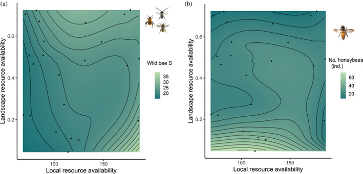
Cities are socioecological systems that filter and select species, therefore establishing unique species assemblages and biotic interactions. Urban ecosystems can host richer wild bee communities than highly intensified agricultural areas, specifically in resource-rich urban green spaces such as allotments and family gardens. At the same time, urban beekeeping has boomed in many European cities, raising concerns that the fast addition of a large number of managed bees could deplete the existing floral resources, triggering competition between wild bees and honeybees. Here, we studied the interplay between resource availability and the number of honeybees at local and landscape scales and how this relationship influences wild bee diversity. We collected wild bees and honeybees in a pollination experiment using four standardized plant species with distinct floral morphologies. We performed the experiment in 23 urban gardens in the city of Zurich (Switzerland), distributed along gradients of urban and local management intensity, and measured functional traits related to resource use. At each site, we quantified the feeding niche partitioning (calculated as the average distance in the multidimensional trait space) between the wild bee community and the honeybee population. Using multilevel structural equation models (SEM), we tested direct and indirect effects of resource availability, urban beekeeping, and wild bees on the community feeding niche partitioning. We found an increase in feeding niche partitioning with increasing wild bee species richness. Moreover, feeding niche partitioning tended to increase in experimental sites with lower resource availability at the landscape scale, which had lower abundances of honeybees. However, beekeeping intensity at the local and landscape scales did not directly influence community feeding niche partitioning or wild bee species richness. In addition, wild bee species richness was positively influenced by local resource availability, whereas local honeybee abundance was positively affected by landscape resource availability. Overall, these results suggest that direct competition for resources was not a main driver of the wild bee community. Due to the key role of resource availability in maintaining a diverse bee community, our study encourages cities to monitor floral resources to better manage urban beekeeping and help support urban pollinators.

Keywords: competition; intraspecific trait variability; pollinator; species interaction; urban biodiversity; urbanization.


Conflict of interest statement

The authors declare no conflict of interest.

Figures

FIGURE 1
FIGURE 1
Illustration of the functional metric and hypotheses regarding the drivers of wild bee community structure. (a) A hypothetical bee community, composed of seven wild bee species (colored circles) and honeybees (blue triangles), depicted in a trait space defined by two traits: intertegular distance (ITD, x‐axis) and relative tongue length (RTL, y‐axis). Three hypotheses are presented regarding the influence of competition (biotic filtering) and environmental filtering in shaping the functional composition of a bee community (b–d) and the feeding niche partitioning between wild bees and honeybees (e). In (b), competition intensity is assumed to be the main driver shaping the wild bee community. Competition intensity can increase as a result of higher beekeeping intensity (larger number of honeybee individuals in a site or hives in the surrounding landscape) and/or lower resource availability. Therefore, with increasing competition intensity, wild bee species that are functionally similar to honeybees (dots inside the gray patch) are expected to be outcompeted and removed from the community due to (excessive) niche overlap. In the opposite scenario (d), a certain environmental gradient (e.g., urbanization intensity) is assumed to be the main driver shaping the wild bee community. Environmental filtering intensity represents environmental drivers that filter traits without necessarily influencing biotic interactions (competition) directly, for example, temperature, habitat loss, and fragmentation. Therefore, with increasing environmental filtering intensity, wild bee species functionally dissimilar to honeybees (dots inside the gray patches) are filtered out, and the best adapted phenotypes under these types of environmental conditions (i.e., those similar to honeybees) dominate the community. In (c), an intermediate scenario is shown, in which both biotic interactions and environment are expected to simultaneously shape the wild bee community. In (e), the changes in the community niche partitioning (defined as the mean pairwise distance of all wild bee individuals with all honeybee individuals) under the different hypotheses are represented in a simplified plot. Thicker lines indicate a major influence of biotic interactions (b), whereas thinner lines indicate that environmental conditions have a larger impact (d). As the two processes are expected to drive feeding niche partitioning in opposite directions, no change may be observed along environmental gradients (c, flat line). Note that, for simplicity, only two traits are depicted in (a–d), whereas only three linear lines are plotted in (e) even though other relationships could occur.
FIGURE 2
FIGURE 2
Final structural equation model (SEM). The SEM model shows the direct and indirect effects of the proxies for resource availability and beekeeping intensity at the landscape and local scale on wild bee diversity proxies, that is, wild bee species richness and the feeding niche partitioning (i.e., the mean pairwise distances between wild bee and honeybee individuals in a given site). The SEM model also includes two models explaining the factors shaping the plant species richness at the local site (proxy of resource availability at the local scale) and the number of honeybee individuals (proxy of beekeeping intensity at the local scale). The thickness of paths has been scaled based on the magnitude of the standardized regression coefficient. Numbers show standardized path coefficients for significant pathways. Positive paths are depicted in black, negative in red, and nonsignificant (p > 0.05) in gray. For each response variable, the R 2 is provided inside the box. AICc = 778.81, Fisher's C = 27.72, p‐value = 0.116. AICc, corrected Akaike information criterion.
FIGURE 3
FIGURE 3
Changes in feeding niche partitioning. Wild bee species composition in relation to feeding niche partitioning value (i.e., the mean pairwise distances between wild bee and honeybee individuals in a given site) at each site. Wild bee species are sorted according to their functional dissimilarity to honeybees, with functionally similar species on the top and functionally dissimilar species on the bottom. The size of each dot represents the proportion of individuals sampled at a given site. Images retrieved from: https://www.flickr.com/people/usgsbiml/.
FIGURE 4
FIGURE 4
(a, b, e, f) Linear models and (c, d) generalized additive models (GAM) with the adjusted R 2 between feeding niche partitioning and resource availability at the landscape scale using as proxy the proportion of green areas at 100 m (a) and 500 m (b); resource availability at the local scale, using as a proxy the plant species richness (c); wild bee species richness (d), and urban beekeeping at the local scale, using as a proxy. The number of honeybee individuals (e); and landscape scale, using as a proxy the number of honeybee hives at 500 m (f). Smooth terms in GAMs are calculated using cubic regression splines. Gray bands indicate 95% confidence intervals. Dots represent the feeding niche partitioning between the wild bee community and the honeybee population at each of the 23 studied gardens. Please refer to Appendix S1: Figures S7–S11 for additional plots depicting the community composition along gradients of beekeeping intensity and resource availability at local and landscape scales. Significance values: *0.01 < p < 0.05.
FIGURE 5
FIGURE 5
Influence of landscape and local resource availability on the number of honeybee individuals and wild bee species richness in the 23 studied gardens. Linear models depicting the relationship between the number of honeybees (a, c, e) and the wild bee species richness (b, d, f) with the proportion of green surfaces in a 500 m radius (a, b) and 100 m radius (c, d), and the local plant species richness (e, f). For each linear model, the adjusted R 2 is provided. Gray bands indicate the 95% confidence intervals. Black dots represent the study gardens. Dots represent each of the 23 studied gardens. S, species richness.
FIGURE 6
FIGURE 6
Contour plots of the predicted number of wild bee species (a) and the number of honeybees (b) with respect to resource availability at the local and landscape scale, showing that wild bee species richness and honeybee abundances are influenced by resource availability at different spatial scales (local and landscape scale, respectively). Contour plots are based on a locally estimated scatterplot smoothing (LOESS) model on the plant species richness (local resource availability) and proportion of green surfaces in a 500 m radius (landscape resource availability). Dots represent each of the 23 studied gardens.

Similar articles

Cited by

References

    1. Albert, C. H. , de Bello F., Boulangeat I., Pellet G., Lavorel S., and Thuiller W.. 2012. “On the Importance of Intraspecific Variability for the Quantification of Functional Diversity.” Oikos 121: 116–26.
    1. Alberti, M. 2015. “Eco‐Evolutionary Dynamics in an Urbanizing Planet.” Trends in Ecology & Evolution 30: 114–26. - PubMed
    1. Baldock, K. C. R. 2020. “Opportunities and Threats for Pollinator Conservation in Global Towns and Cities.” Current Opinion in Insect Science 38: 63–71. - PubMed
    1. Baldock, K. C. R. , Goddard M. A., Hicks D. M., Kunin W. E., Mitschunas N., Morse H., Osgathorpe L. M., et al. 2019. “A Systems Approach Reveals Urban Pollinator Hotspots and Conservation Opportunities.” Nature Ecology and Evolution 3: 363–73. - PMC - PubMed
    1. Baldock, K. C. R. , Goddard M. A., Hicks D. M., Kunin W. E., Mitschunas N., Osgathorpe L. M., Potts S. G., et al. 2015. “Where is the UK's Pollinator Biodiversity? The Importance of Urban Areas for Flower‐Visiting Insects.” Proceedings of the Royal Society B: Biological Sciences 282(1803): 20142849. 10.1098/rspb.2014.2849. - DOI - PMC - PubMed

Publication types

LinkOut - more resources