The trend of disruption in the functional brain network topology of Alzheimer's disease

Abstract

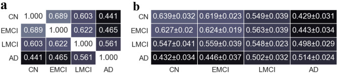
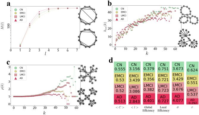
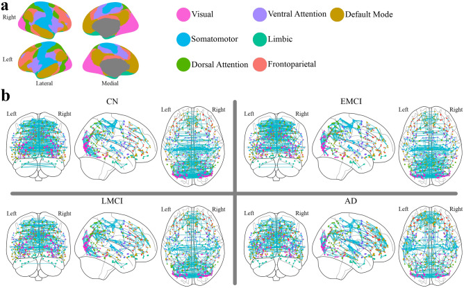
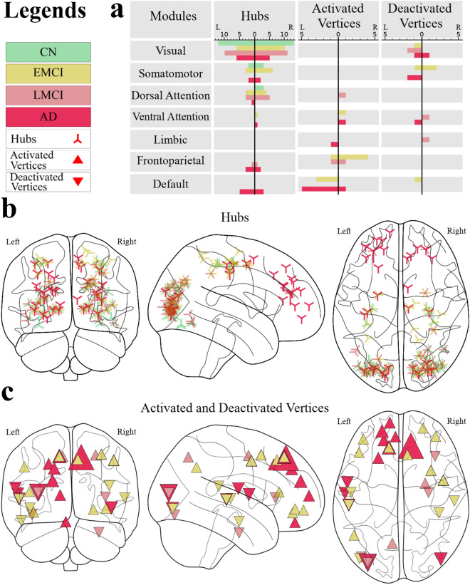
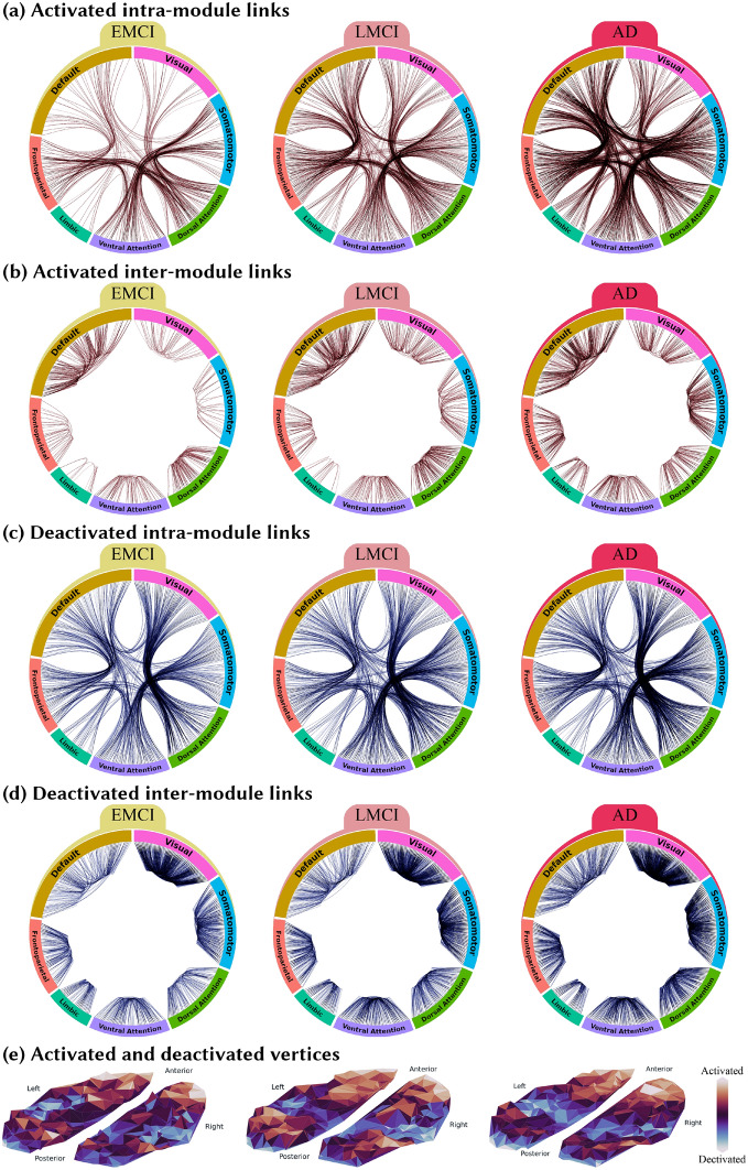
Alzheimer's disease (AD) is a progressive disorder associated with cognitive dysfunction that alters the brain's functional connectivity. Assessing these alterations has become a topic of increasing interest. However, a few studies have examined different stages of AD from a complex network perspective that cover different topological scales. This study used resting state fMRI data to analyze the trend of functional connectivity alterations from a cognitively normal (CN) state through early and late mild cognitive impairment (EMCI and LMCI) and to Alzheimer's disease. The analyses had been done at the local (hubs and activated links and areas), meso (clustering, assortativity, and rich-club), and global (small-world, small-worldness, and efficiency) topological scales. The results showed that the trends of changes in the topological architecture of the functional brain network were not entirely proportional to the AD progression. There were network characteristics that have changed non-linearly regarding the disease progression, especially at the earliest stage of the disease, i.e., EMCI. Further, it has been indicated that the diseased groups engaged somatomotor, frontoparietal, and default mode modules compared to the CN group. The diseased groups also shifted the functional network towards more random architecture. In the end, the methods introduced in this paper enable us to gain an extensive understanding of the pathological changes of the AD process.

Figure 1

The similarity between study groups follows a trend proportional to the trend of disease progression. (a) The Jaccard similarity coefficient between the four main group networks. (b) For each study group, the 23 subjects of each group were randomly divided into two subgroups of 11 and 12 networks. Then, the mean networks of these 12 and 11 subjects were constructed, and the Jaccard similarity coefficient between these two mean networks was computed. This process was repeated 100 times resulting in 100 Jaccard similarity coefficient matrices. This panel shows the element-wise mean and SD of these matrices.

Figure 2

The emergence of the small-worldness, assortativity, and rich-club phenomenon in the group networks. (a) M(l) plot showing the average number of vertices within a distance less than or equal to l from any given vertex is almost increased by the disease progression and suggests that the group networks have the small-world property that is almost stronger in the disease networks. Two graphs on the right-hand side are toy examples to provide intuition on the relationship between the small-world property and randomness, demonstrating the increase in the randomness of network connections (from bottom to top), which leads to the increase in the emergence of the small-world property. The bottom network is more regular, whereas the top one is more random. As a result, the average shortest path length is shorter in the random network (top) than the regular one (bottom), causing the regular network to be less small-world. (b) $K_{\mathit{nn}}(k)$ plot showing the average degree of the nearest neighbors, for vertices of degree k, is almost decreased by the disease progression and suggests that the group networks have assortative architecture, and this assortative matching follows a decreasing trend proportional to the disease progression. Two graphs on the right-hand side are toy examples of assortative (top) and disassortative (bottom) networks to provide intuition on the assortative patterns. As it is obvious, in the bottom network, high degree vertices are more connected with low degree vertices (disassortative pattern), whereas, in the top network, its vertices tend to make connections with other vertices that have similar degrees (assortative pattern). (c) $\rho (k)$ plot showing the amount of inter-connectivity among vertices of degree higher than k is almost decreased by the disease progression and suggests that the rich-club phenomenon is disappearing by the disease progression. Two graphs on the right-hand side are toy examples of networks with (top) and without (bottom) rich-club. In the bottom network, there is no significant inter-connectivity among high-degree vertices (rich vertices). However, in the top network, which is an example of a rich-club network, high-degree vertices are completely inter-connected. (d) The bar plots showing $<C>$, $<l>$, global efficiency, local efficiency, $\sigma$ (normalized $<C>$/ normalized $<l>$), and r (PCC between the degrees of all vertices at either ends of a link).

Figure 3

The overall gradually changing patterns of highly-weighted links are following a trend proportional to the disease progression. (a) The spatial distribution of the 7-module parcellation. (b) The top 1 percent highly-weighted links of each group network. Vertex color represents the module the vertex belongs to, and the vertex size is proportional to the vertex strength. It shows that there is a trend towards the increase in the number of default mode links as well as the decrease in the inter-hemisphere links in dorsal attention. Visualizations were created using ggseg 1.6.1 R package (a) and Nilearn 0.6.2 (https://nilearn.github.io) (b).

Figure 4

The distribution of hubs, activated areas, and deactivated areas shows that anterior regions are more engaged in the diseased groups. (a) The frequency distribution across the 7-module parcellation. The left and right sides of each sub-plot denoted by a vertical black line represent the distribution across modules limited to the left and right hemispheres, respectively (b) The spatial distribution of the hub regions. The vertex size is proportional to the vertex strength. (c) The spatial distribution of vertices that are activated (denoted by $△$) and deactivated (denoted by $▽$) in the diseases. A vertex was called activated (deactivated) with respect to disease if the subtraction of its strength in the disease network from the CN network was significantly larger (smaller) than the similar value for other vertices. The vertex size is proportional to the value of this subtraction. Visualizations in (b) and (c) were created using Nilearn package.

Figure 5

The alterations in the brain functional network induced by the disease progression. For each disease stage, the connectogram of the links with significantly higher (activated) or lower (deactivated) weights compared to the CN group is depicted in the top four panels: (a) connectogram of intra-module links activated in each disease stage compared to the CN group, (b) Connectogram of inter-module links activated in each disease stage compared to the CN group, (c) connectogram of intra-module links deactivated in each disease stage compared to the CN group, and (d) Connectogram of inter-module links deactivated in each disease stage compared to the CN group. For each disease group, the activated (deactivated) links compared to the CN group are defined as the significantly larger (smaller) elements of the matrix resulting from the subtraction of the disease network from the CN network. Diagrams are plotted based on the Hierarchical Edge Bundling algorithm using ObservableHQ platform (https://observablehq.com). This algorithm allows bundling the intra-module links to get a more elegant presentation. Panel (e) indicates the activation or deactivation in the vertices’ strength by showing the top-view spatial distribution of the activated or deactivated vertices similar to Fig. 4c.

References

1. 2020 alzheimer’s disease facts and figures. Alzheimer’s & Dementia16, 391–460. 10.1002/alz.12068. https://alz-journals.onlinelibrary.wiley.com/doi/pdf/10.1002/alz.12068. - DOI - PubMed
1. Organization, W. H. Global Tuberculosis Report 2019. Global tuberculosis control (World Health Organization, 2019).
1. Davis M, et al. Estimating alzheimer’s disease progression rates from normal cognition through mild cognitive impairment and stages of dementia. Curr. Alzheimer Res. 2018;15:777–788. doi: 10.2174/1567205015666180119092427. - DOI - PMC - PubMed
1. Supekar K, Menon V, Rubin D, Musen M, Greicius MD. Network analysis of intrinsic functional brain connectivity in alzheimer’s disease. PLoS Comput. Biol. 2008;4:e1000100. doi: 10.1371/journal.pcbi.1000100. - DOI - PMC - PubMed
1. Zhou J, et al. Divergent network connectivity changes in behavioural variant frontotemporal dementia and alzheimer’s disease. Brain. 2010;133:1352–1367. doi: 10.1093/brain/awq075. - DOI - PMC - PubMed
Publication types