Attractive serial dependence overcomes repulsive neuronal adaptation

Abstract

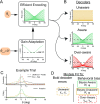
Sensory responses and behavior are strongly shaped by stimulus history. For example, perceptual reports are sometimes biased toward previously viewed stimuli (serial dependence). While behavioral studies have pointed to both perceptual and postperceptual origins of this phenomenon, neural data that could elucidate where these biases emerge is limited. We recorded functional magnetic resonance imaging (fMRI) responses while human participants (male and female) performed a delayed orientation discrimination task. While behavioral reports were attracted to the previous stimulus, response patterns in visual cortex were repelled. We reconciled these opposing neural and behavioral biases using a model where both sensory encoding and readout are shaped by stimulus history. First, neural adaptation reduces redundancy at encoding and leads to the repulsive biases that we observed in visual cortex. Second, our modeling work suggest that serial dependence is induced by readout mechanisms that account for adaptation in visual cortex. According to this account, the visual system can simultaneously improve efficiency via adaptation while still optimizing behavior based on the temporal structure of natural stimuli.

Fig 1. Caption behavior.

(A) Task schematic. An orientated stimulus is followed by a probe bar that is rotated <15° from the stimulus. Participants judged whether the bar was CW or CCW relative to the stimulus in a binary discrimination task. (B) Response bias: % of responses that were CCW as a function of Δθ = θn − 1 − θn (± SEM across participants). (C) Behavioral bias, green: average model-estimated bias as a function of Δθ (± SEM across participants); gray: average DoG fit to raw participant responses sorted by Δθ (± 1SEM across participants). (D) Response accuracy as a function of Δθ. (E) Responses are significantly more accurate for |Δθ|<30°. (F) Behavioral σ as a function of Δθ. (G) Behavioral variance is significantly less for |Δθ|<30°. Note that in computing variance, we “flip” the sign of errors following CCW inducing trials to avoid conflating bias with variance (see Methods). (H) Bias is positively correlated with variance across participants. ***, p < 0.001. Data and code supporting this figure found here: https://osf.io/e5xw8/?view_only=e7c1da85aa684cc8830aec8d74afdcb4. CCW, counterclockwise; CW, clockwise.

Fig 2. Caption behavioral and neural bias.

(A) Left axis, behavioral serial dependence. Shaded green: average model-estimated bias as a function of Δθ (± SEM across participants); dotted black line: average DoG fit to raw participant responses sorted by Δθ. Right axis, variance. Purple shaded line: model-estimated variance as a function of Δθ (± SEM across participants). (B) Behavioral σ is significantly less for |Δθ|<30°. (C) Decoded orientation was significantly greater than chance when indexed with circular correlation for all ROIs examined. Error bars indicate ±SEM across participants. Dots show data from individual participants. (D) Decoding performance across time for a subset of ROIs. Vertical red line indicates time point used in most analysis. (E) Decoding performance across time for a decoder trained on a separate sensory localization task. (F) Performance of task decoder trained and tested on identity of previous stimulus across all ROIs. (G) Left axis, decoding bias. Shaded yellow line: decoded bias (μ_circ of decoding errors) sorted by Δθ (± SEM across participants); dotted black line: average DoG fit to raw decoding errors sorted by Δθ. Right axis, decoded σ_circ. Shaded gray line: average decoding variance (σ_circ) as a function of Δθ (± SEM across participants). Note that σ_circ can range from [0, inf] and has no units. (H) Decoded variance is significantly greater for |Δθ|<30°. (I) Decoded errors are significantly repulsive when parameterized with a DoG in all ROIs. *, p < 0.05; **, p < 0.01; ***, p < 0.001. Data and code supporting this figure found here: https://osf.io/e5xw8/?view_only=e7c1da85aa684cc8830aec8d74afdcb4. DoG, Derivative of Gaussian; ROI, region of interest.

Fig 3. Influence of BOLD-specific biases on repulsive bias.

(A) Average V1 HRF through deconvolution for stimulus and probe. Average best fit double gamma function overlaid in dotted lines. (B) (Left) Bias curves from decoder trained on response patterns from deconvolved double-gamma functions (± SEM across participants). Here excluding hV4 and IPS0 for clarity. (Right) Bias quantified with a DoG function across ROIs. (C) Bias across time including only trials with an ISI of at least 17.5 seconds. x-Axis reflects minimum time from previous stimulus. Repulsion significant in all ROIs at 32 seconds. (D) Bias as a function of various relative orientations for V1 and V3 (± SEM across participants). (E) Bias across early visual ROIs for N-1, N-2, and N-3. Color scheme same as C. N+1 control analysis to ensure effects not driven by some unknown structure in stimulus sequence. (F) Behavioral bias for various relative orientations. N-1 data same as data presented in Fig 2. *, p < 0.05, **, p < 0.01, ***, p < 0.001. Data and code supporting this figure found here: https://osf.io/e5xw8/?view_only=e7c1da85aa684cc8830aec8d74afdcb4. DoG, Derivative of Gaussian; HRF, hemodynamic response function; ROI, region of interest.

Fig 4. Encoder–decoder model schematic.

(A) Encoding. Units with von Mises tuning curves encodes incoming stimuli. The gain of individual units undergoes adaptation such that their activity is reduced as a function of their distance from the previous stimulus. (B) Decoding. This activity is then read out using a scheme that assumes 1 of 3 adaptation profiles. The unaware decoder assumes no adaptation has taken place, the aware decoder assumes the true amount of adaptation while the overaware decoder overestimates the amount of adaptation (note center tuning curves dip lower than the minimum gain line from encoding). (C) Example stimulus decoding. Top: The resulting likelihood function for the unaware readout (dotted yellow line) has its representation for the current trial (θ_n = −30°) biased away from the previous stimulus (θ_n-1 = 0°). The aware readout (dotted green line) is not biased, while the overaware readout is biased toward the previous stimulus. These likelihood functions can be multiplied by a prior of stimulus contiguity (solid black line) to get a Bayesian posterior (bottom) where Bayes-unaware and Bayes-aware representations are shifted toward the previous stimulus. Tick marks indicate maximum likelihood or decoded orientation. (D) Summary of models and free parameters being fit to both BOLD decoder errors and behavioral bias. Data and code supporting this figure found here: https://osf.io/e5xw8/?view_only=e7c1da85aa684cc8830aec8d74afdcb4.

Fig 5. Model performance bias.

(A–C) Neural/behavioral bias. (D–G) Neural/behavioral variance. (A) Unaware decoder (yellow) provides a good fit to neural bias (black outline). Decoded variance decreases monotonically with distance from previous stimulus. (± SEM across participants). (B) Perceptual bias (black outline) was well fit by the Bayes-aware and overaware models but not the Bayes-Unaware model (± SEM across participants). (C) Participant responses were significantly more likely under aware models. (D) Behavioral variance had a similar shape and magnitude to Bayes-aware and overaware model fits. Bayes-unaware model output was much less precise and had a different form. (E) Distribution of empirically predicted response errors (black line) and simulated model fits for an example participant. (F) The unaware model’s error distribution had significantly higher Jenson–Shannon divergence from BOLD decoder than either aware model. (G) Visualization of all uncertainties split as a function of close and far stimuli. Note that the Bayes-unaware model had an average uncertainty that was on average 6x that of perception. *, p < 0.05; **, p < 0.01; ***, p < 0.001. Data and code supporting this figure found here: https://osf.io/e5xw8/?view_only=e7c1da85aa684cc8830aec8d74afdcb4.

References

1. Dong DW, Atick JJ. Statistics of natural time-varying images. Netw Comput Neural Syst. 1995; 6(3):345–58.
1. Felsen G, Touryan J, Dan Y. Contextual modulation of orientation tuning contributes to efficient processing of natural stimuli. Netw Comput Neural Syst. 2005; 16(2–3):139–49. doi: 10.1080/09548980500463347 - DOI - PubMed
1. Girshick AR, Landy MS, Simoncelli EP. Cardinal rules: visual orientation perception reflects knowledge of environmental statistics. Nat Neurosci. 2011; 14(7):926–32. doi: 10.1038/nn.2831 - DOI - PMC - PubMed
1. van Bergen RS, Jehee JFM. Probabilistic Representation in Human Visual Cortex Reflects Uncertainty in Serial Decisions. J Neurosci. 2019; 39(41):8164–76. doi: 10.1523/JNEUROSCI.3212-18.2019 - DOI - PMC - PubMed
1. Dragoi V, Rivadulla C, Sur M. Foci of orientation plasticity in visual cortex. Nature. 2001; 411(6833):80–6. doi: 10.1038/35075070 - DOI - PubMed
Publication types