Pump-probe capabilities at the SPB/SFX instrument of the European XFEL

Abstract

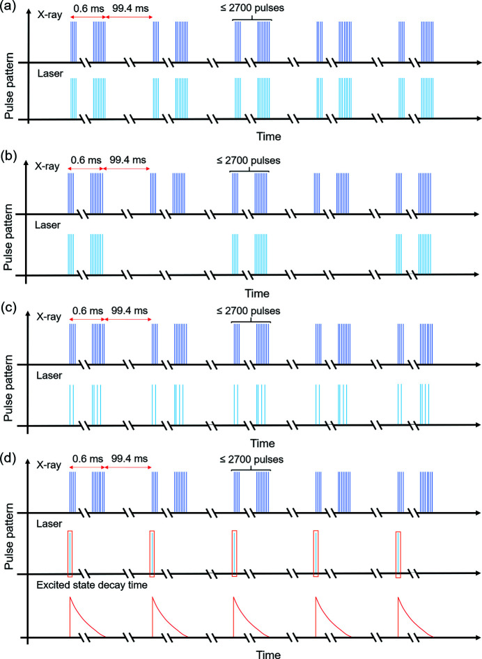
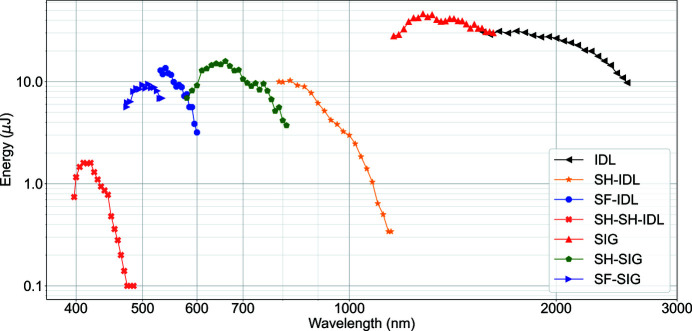
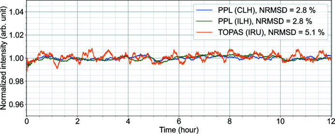
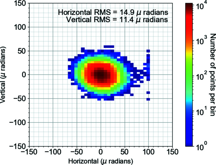
Pump-probe experiments at X-ray free-electron laser (XFEL) facilities are a powerful tool for studying dynamics at ultrafast and longer timescales. Observing the dynamics in diverse scientific cases requires optical laser systems with a wide range of wavelength, flexible pulse sequences and different pulse durations, especially in the pump source. Here, the pump-probe instrumentation available for measurements at the Single Particles, Clusters, and Biomolecules and Serial Femtosecond Crystallography (SPB/SFX) instrument of the European XFEL is reported. The temporal and spatial stability of this instrumentation is also presented.

Keywords: European XFEL; megahertz pump and probe sources; pump–probe experiments; time-resolved experiments.

Figure 1

Top view of the general layout of the SPB/SFX instrument showing the central laser hutch, instrument laser hutch and experiment hutch. The two interactions regions are highlighted by orange boxes, the PP laser beam pipes and beam directions are marked in red, and the X-ray beam, marked in violet, goes from left to right.

Figure 2

Schematic of a pump–probe experimental setup at IRU of the SPB/SFX instrument.

Figure 3

Spectral (a) and temporal (b) profile of the PP laser at 15 fs FWHM and 50 fs FWHM pulse duration. The insets show the beam profile in the near-field (c) and far-field (d).

Figure 4

Visualizing the water jet explosion induced by an intense X-ray pulse with the PP laser. The image was captured by the side microscope with a 20× objective (20× Mitutoyo Plan Apo SL Infinity Corrected Objective, 378-810-3).

Figure 5

Several examples of pulse pattern setting for optical laser pulses. (a) Pump and probe source have the same pulse pattern. (b) Burst-mode operation where the optical laser pulses are down picked for so-called light and dark states for consecutive trains. (c) Burst-mode excitation with an arbitrary intra-train pulse pattern derived from a megahertz X-ray pulse pattern. (d) 10 Hz pump and sampling with a megahertz X-ray pulse pattern.

Figure 6

Output of TOPAS at different wavelengths. For this measurement, TOPAS was pumped by the PP laser with the following parameters: 800 nm, ∼54 fs, 215 µJ and 50 pulses per train at 1.1 MHz. (SH – second harmonic; SF – sum frequency; SIG – signal; IDL – idler).

Figure 7

Intensity stability of the TOPAS output measured at IRU over 12 h with the output beam set at a wavelength of 640 nm. The three lines show the 10 min moving average of intensity stability of the PP laser in the CLH, the ILH and the OPA output at IRU. Here the intensity is normalized to the mean intensity of each measurement.

Figure 8

2D histogram of the pointing stability of the TOPAS output beam in the horizontal and vertical directions.

Figure 9

Double exposure stroboscopic imaging of droplets with two nanosecond lasers with a delay of hundreds of nanoseconds between the two pulses. A zoomed view of one of the droplets imaged is shown in the inset. The image was collected using the side microscope with a 10× objective and an Andor Zyla 5.5 camera.

Figure 10

An aerosol particle beam with particles of size of a few tens of nanometres visualized by Rayleigh scattering imaging using the (a) inline microscope with 10× objective and (b) side microscope with 2× objective.

Figure 11

Schematic of (a) the PAM setup, and (b) the PAM sample holder.

Figure 12

Plot of temporal jitter measured over 15 min. The darker blue line shows the rolling mean over 5 s (Sato et al., 2020 ▸).

Figure 13

Time zero position determination using spatial encoding at SPB/SFX. (a) Laser transmission imaged with the side microscope with 10× magnification. (b) Line-out of the selected region highlighted by the white box in (a).

References

-
- Allahgholi, A., Becker, J., Bianco, L., Delfs, A., Dinapoli, R., Goettlicher, P., Graafsma, H., Greiffenberg, D., Hirsemann, H., Jack, S., Klanner, R., Klyuev, A., Krueger, H., Lange, S., Marras, A., Mezza, D., Mozzanica, A., Rah, S., Xia, Q., Schmitt, B., Schwandt, J., Sheviakov, I., Shi, X., Smoljanin, S., Trunk, U., Zhang, J. & Zimmer, M. (2015). J. Instrum. 10, C01023.
- Ayyer, K., Xavier, P. L., Bielecki, J., Shen, Z., Daurer, B. J., Samanta, A. K., Awel, S., Bean, R., Barty, A., Bergemann, M., Ekeberg, T., Estillore, A. D., Fangohr, H., Giewekemeyer, K., Hunter, M. S., Karnevskiy, M., Kirian, R. A., Kirkwood, H., Kim, Y., Koliyadu, J., Lange, H., Letrun, R., Lübke, J., Michelat, T., Morgan, A. J., Roth, N., Sato, T., Sikorski, M., Schulz, F., Spence, J. C. H., Vagovic, P., Wollweber, T., Worbs, L., Yefanov, O., Zhuang, Y., Maia, F. R. N. C., Horke, D. A., Küpper, J., Loh, N. D., Mancuso, A. P. & Chapman, H. N. (2021). Optica, 8, 15–23.
- Bean, R. J., Aquila, A., Samoylova, L. & Mancuso, A. P. (2016). J. Opt. 18, 074011.
- Biasin, E., Fox, Z. W., Andersen, A., Ledbetter, K., Kjaer, K. S., Alonso-Mori, R., Carlstad, J. M., Chollet, M., Gaynor, J. D., Glownia, J. M., Hong, K., Kroll, T., Lee, J. H., Liekhus-Schmaltz, C., Reinhard, M., Sokaras, D., Zhang, Y., Doumy, G., March, A. M., Southworth, S. H., Mukamel, S., Gaffney, K. J., Schoenlein, R. W., Govind, N., Cordones, A. A. & Khalil, M. (2021). Nat. Chem. 13, 343–349.
- Bielecki, J., Hantke, M. F., Daurer, B. J., Reddy, H. K. N., Hasse, D., Larsson, D. S. D., Gunn, L. H., Svenda, M., Munke, A., Sellberg, J. A., Flueckiger, L., Pietrini, A., Nettelblad, C., Lundholm, I., Carlsson, G., Okamoto, K., Timneanu, N., Westphal, D., Kulyk, O., Higashiura, A., van der Schot, G., Loh, N. D., Wysong, T. E., Bostedt, C., Gorkhover, T., Iwan, B., Seibert, M. M., Osipov, T., Walter, P., Hart, P., Bucher, M., Ulmer, A., Ray, D., Carini, G., Ferguson, K. R., Andersson, I., Andreasson, J., Hajdu, J. & Maia, F. R. N. C. (2019). Sci. Adv. 5, eaav8801. - PMC - PubMed
MeSH terms
Grants and funding
LinkOut - more resources
Full Text Sources