Constructing functional models from biophysically-detailed neurons

Abstract

Improving biological plausibility and functional capacity are two important goals for brain models that connect low-level neural details to high-level behavioral phenomena. We develop a method called "oracle-supervised Neural Engineering Framework" (osNEF) to train biologically-detailed spiking neural networks that realize a variety of cognitively-relevant dynamical systems. Specifically, we train networks to perform computations that are commonly found in cognitive systems (communication, multiplication, harmonic oscillation, and gated working memory) using four distinct neuron models (leaky-integrate-and-fire neurons, Izhikevich neurons, 4-dimensional nonlinear point neurons, and 4-compartment, 6-ion-channel layer-V pyramidal cell reconstructions) connected with various synaptic models (current-based synapses, conductance-based synapses, and voltage-gated synapses). We show that osNEF networks exhibit the target dynamics by accounting for nonlinearities present within the neuron models: performance is comparable across all four systems and all four neuron models, with variance proportional to task and neuron model complexity. We also apply osNEF to build a model of working memory that performs a delayed response task using a combination of pyramidal cells and inhibitory interneurons connected with NMDA and GABA synapses. The baseline performance and forgetting rate of the model are consistent with animal data from delayed match-to-sample tasks (DMTST): we observe a baseline performance of 95% and exponential forgetting with time constant τ = 8.5s, while a recent meta-analysis of DMTST performance across species observed baseline performances of 58 - 99% and exponential forgetting with time constants of τ = 2.4 - 71s. These results demonstrate that osNEF can train functional brain models using biologically-detailed components and open new avenues for investigating the relationship between biophysical mechanisms and functional capabilities.

Fig 1. Target tuning curve distribution.

An example of the distribution of responses for 100 ReLU neurons with x-intercepts in -[1, 1] and y-intercepts in [20, 40].

Fig 2. Network used during osNEF training.

The top half of the figure is the “oracle” stream, where the desired filters and transformations are applied analytically, and where the target activities are generated. The bottom half of the figure is the “network” stream, where synaptic connections realize the desired filters and transformations, and where osNEF training is applied to update the relevant synaptic parameters. Both streams are driven by an input x (we omit all time-dependencies, such as x(t) and J(t), for brevity). Arrows represent the signal travelling through each stream. Boxes letters (filters h, weights w, transformations I, and decoders d) indicate mathematical operations being applied to the signal. The resulting quantities (spikes δ, synaptic currents J, synaptic conductances σ, and states x) are shown above the arrow. The pink numbers reference Table 1, which lists the operations that are applied at each step. Circled abbreviations indicate neural populations, which receive synaptic inputs and produce spikes. Coloration indicates ReLU neurons (gray) or detailed neurons (blue), parameters updated by osNEF’s online learning rules (orange) or offline synaptic optimization (green), references (pink), and NEF operations (gray).

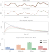
Fig 3. Encoding and tuning curves.

The top panel shows the input signal and the target x-intercept, the state space value at which our neurons should begin spiking. The middle panel shows neural activity over time and the target y-intercept, the desired activity of our neurons when the input is at its maximum value. The bottom panel shows the tuning curves derived from these data. All four neuron models exhibit minimal spiking activity when the input is below the target x-intercept; neural activities also increase as the value of the input increases, up to the target y-intercept. Shaded error regions indicate 95% confidence intervals for smoothed activity, and demonstrate that all simulated neuron models have a natural variation in firing rate for any given state space value x. The significant overlap between the four trained neuron models and the target (ReLU) activities shows the success of our online learning rule.

Fig 4. Decoding and readout filters.

Nonlinear dynamics within complex neuron models leads to systematic decoding error if a default filter is used to smooth the spikes. Optimizing a filter’s time constants accounts for this problem and reduces spike noise, leading to highly accurate estimates across all neuron models. The top two panels show the target values and the state space estimates, which are decoded from the activities of 100 LIF, Izhikevich, Wilson, or Pyramidal neurons in “pop”; spikes are smoothed using either the default filter (first panel) or the osNEF-trained filter (second panel). The third panel confirms that the RMSE between state space targets and decoded estimates (averaged across 10 simulations with unique inputs) are significantly lower when using the trained filter. The fourth panel shows the impulse response functions.

Fig 5. Network architecture for computing feedforward functions, including the identity function and multiplication of two input scalars.

This network extends the training network in Fig 2, represented by components with the gray background, by including an additional detailed neuron population “pop₂” and the corresponding oracle components. With this architecture, we can compute the feedforward function f(x) on the connection between “pop₁” and “pop₂” by using osNEF to train the synaptic parameters d₁, e₂, and h₁. As before, coloration indicates ReLU neurons (gray) or detailed neurons (blue), synaptic parameters trained by online learning (orange) or offline optimization (green), NEF computations (gray), and finally the new components involved in the calculation of f(x) (purple).

Fig 6. Computing the identity function, Eq 11.

Using the network architecture in Fig 5, we initialize neural populations “pop₁” and “pop₂” with 100 detailed neurons, then use osNEF to train encoders, decoders, and synaptic filters. The connection between “pop₁” and “pop₂” is trained to compute the identity function, such that “pop₂” represents the same information as “pop₁”. The top plot shows the state space target and the decoded estimates from “pop₂”, and the bottom plot shows the mean error (RMSE) between this estimate and the target across 10 simulations with unique input signals.

Fig 7. Computing the product of two unique input signals, Eq 12.

Using the network architecture in Fig 5, we initialize neural populations “pop₁” and “pop₂” with 100 detailed neurons, then use osNEF to train encoders, decoders, and synaptic filters. The connection between “pop₁” and “pop₂” is trained to multiply two scalars: “pop₁” represents the two scalars, and “pop₂” should represent their product. The top plot shows the state space target and the decoded estimates from “pop₂”, and the bottom plot shows the mean error between this estimate and the target across 10 simulations with unique input signals.

Fig 8. Network architecture for recurrent networks.

Orange components indicate the feedforward computation of $\dot{\mathbf{x}}=B\mathbf{u}$, and purple components indicate the recurrent computation of $\dot{\mathbf{x}}=A\mathbf{x}$; together they implement Eq 6. While this network is used at test-time, an “unrolled” version similar to Fig 5 is used during training. As such, we remove reference to “tar”, and to the decoders and encoders composing w, in this figure.

Fig 9. Implementing a simple harmonic oscillator (Eq 13) using a recurrent connection.

Using the network architecture in Fig 5, we initialize neural populations “pop₁” and “pop₂” with 100 detailed neurons, then use osNEF to train encoders, decoders, and synaptic filters. The connection between “pop₁” and “pop₂” is trained to compute Eq 13. The weights and synapses from this trained model are then substituted into a testing network, shown in Fig 8. The top panel shows the state space target and the decoded estimates from “pop₂”, with a break in the x-axis to show that oscillations remain stable over 100 seconds. The bottom panel show the mean error between this estimate and a best-fit sinuoid, as well as the frequency error between this best-fit sinusoid and the target frequency ω = 2π.

Fig 10. Network architecture for the gated difference memory.

This system loads and stores a two-dimensional value in a working memory; when the “gate” signal is on (closed), the system maintains its current value through recurrent activity, and when the “gate” is off (open), the system replaces its current representation with the input value. Gray circles are LIF populations while blue circles are detailed neuron populations. The green connection is trained by osNEF to compute f(x) = x, while the purple connection is trained to compute f(x) = −x. The orange connection directly inhibits neurons in “diff” using fixed negative weights.

Fig 11. Implementing a gated difference memory using a combination of feedfoward, recurrent, feedback, and inhibitory connections.

The left panel shows the estimate decoded from “pop” as a trajectory in (x, y) space: as the cue is presented, the estimate travels from the origin (t = 0) to the cue’s location, which lies somewhere on the unit circle. At t = 1 the cue is removed, and the system must rely on its recurrent dynamics to maintain a stable estimate of the cue’s location. We observe minimal drift in the decoded trajectories for most cue locations, indicating that our memories are fairly stable over time. The right panel shows the Euclidean distance between the decoded estimate and the cue’s true location, averaged over a 10s delay period and over 10 cue locations, for each neuron model.

Fig 12. Architecture for the biologically-constrainted DRT neural network.

This network extends Fig 10 by (a) replacing “inh” with a population of detailed inhibitory interneurons, (b) adding a “cleanup” network that uses WTA competition to find the cue location that best resembles the recalled location from “pop” (see [26] for a detailed description), and (c) replacing all connections to/from detailed neurons with conductance-based AMPA, GABA, or (voltage-gated) NMDA synapses. Grey populations contain LIF neurons, orange populations are interneurons, and blue populations are pyramidal cells. Pink connections use AMPA synapses, orange connections GABA synapses, and green connections use NMDA synapses.

Fig 13. Mnemonic performance of the biologically-detailed cognitive network and the best fit exponential forgetting curve.

We trained the network show in Fig 12 using osNEF to produce a gated difference memory, as described in Sec 4.2 and Fig 10. Rather than average the error over time, as we did in the right panel of Fig 11, we plotted error (percentage of correct responses over 8 cue locations) as a function of time. We repeated this training and testing procedure for ten networks seeds, treating each network as an individual “participant” performing this task, then fit an exponential function to each network’s forgetting curve. From these fitted curves, we obtained parameters for baseline performance and performance half-life, which we compared with the empirical data shown in Fig 14.

Fig 14. Estimated zero-delay performance (left) and performance half-life (right) in DMTST across species.

Performance half-life is defined as the delay for which performance drops from its zero-delay value to a value halfway toward chance performance. Open circles are species medians. Empirical data are taken from [30]. We observe significant differences in the rate of forgetting (performance half-life) between individual networks, a trend that we also observe between individual animals (or experiments) within the empirical data. While the median mnemonic performance of our networks is lower than the median performance of most species in [30], our high-performing networks still outperform a significant number of individual monkeys, rodents, and birds, suggesting that our cognitive networks operate in a biologically plausible WM regime.

References

1. Anderson JR, Lebiere CJ. The atomic components of thought. Psychology Press; 2014.
1. Markram H, Muller E, Ramaswamy S, Reimann MW, Abdellah M, Sanchez CA, et al.. Reconstruction and simulation of neocortical microcircuitry. Cell. 2015;163(2):456–492. doi: 10.1016/j.cell.2015.09.029 - DOI - PubMed
1. Eliasmith C, Stewart TC, Choo X, Bekolay T, DeWolf T, Tang Y, et al.. A large-scale model of the functioning brain. science. 2012;338(6111):1202–1205. doi: 10.1126/science.1225266 - DOI - PubMed
1. Eliasmith C, Anderson CH. Neural engineering: Computation, representation, and dynamics in neurobiological systems. MIT press; 2004.
1. Eliasmith C. How to build a brain: A neural architecture for biological cognition. Oxford University Press; 2013.
Publication types