DEVELOPMENT OF FIBRIN BRANCH STRUCTURE BEFORE AND AFTER GELATION

Abstract

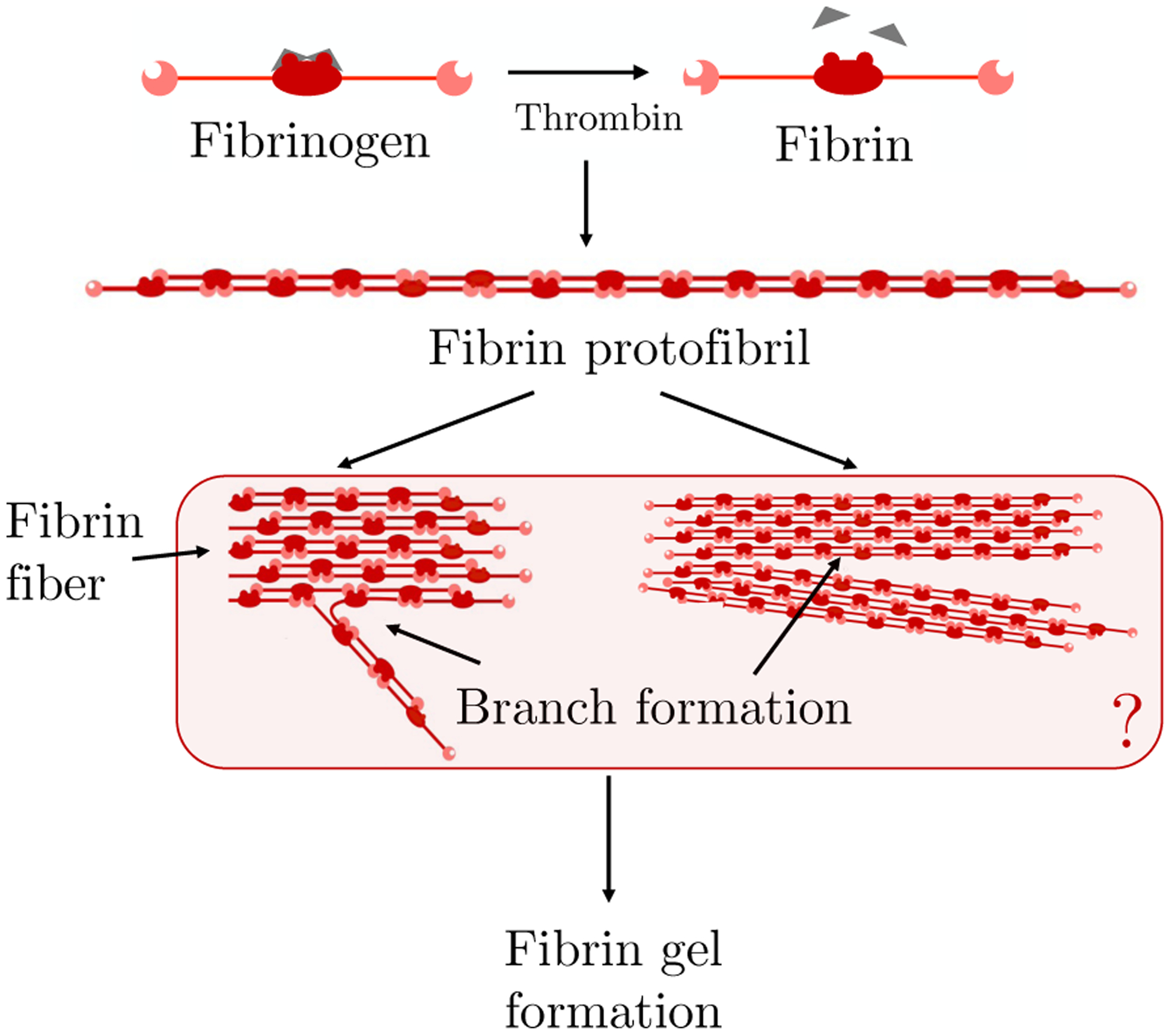
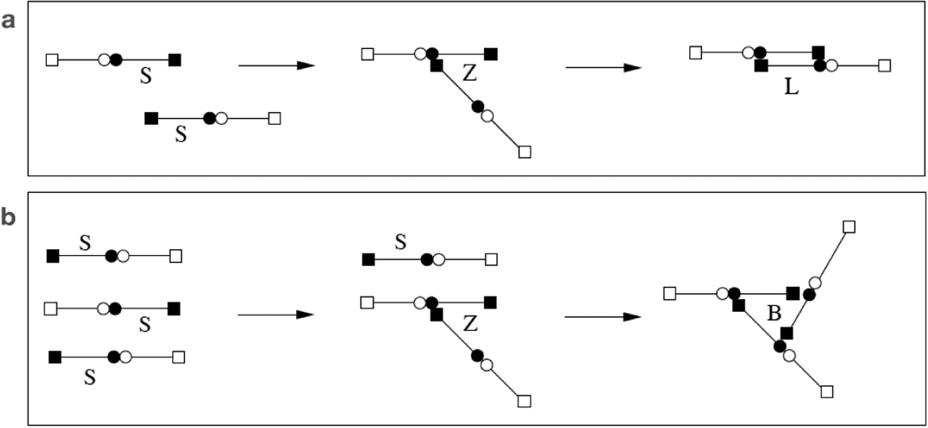
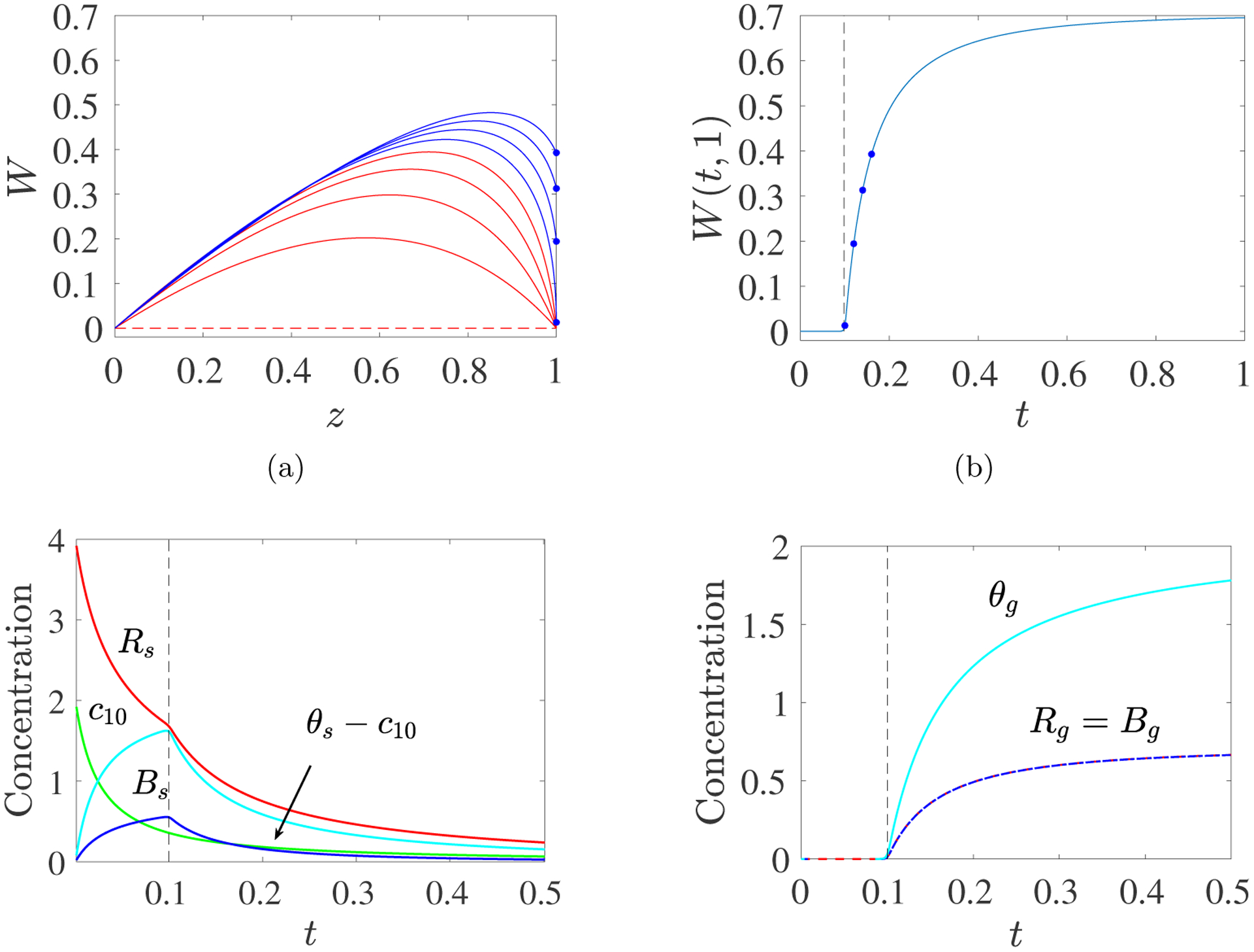
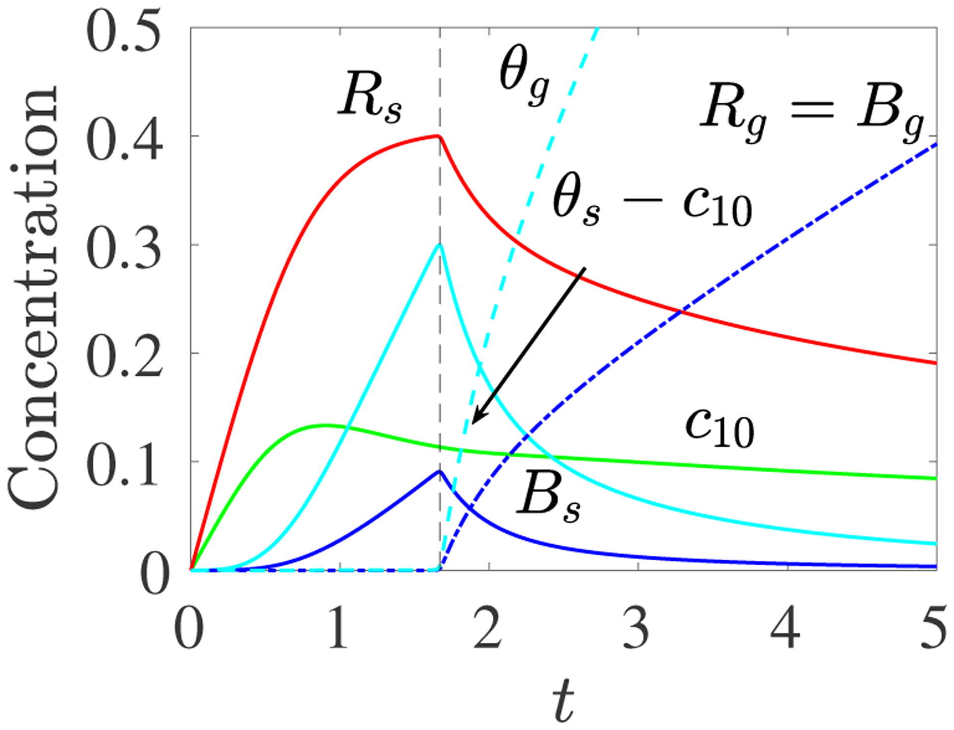
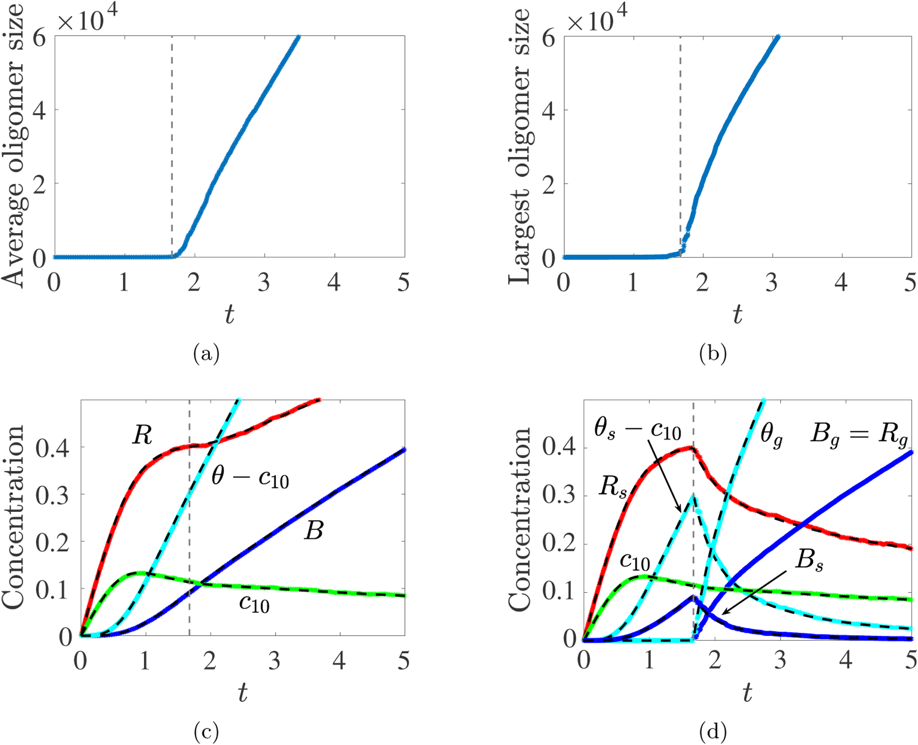
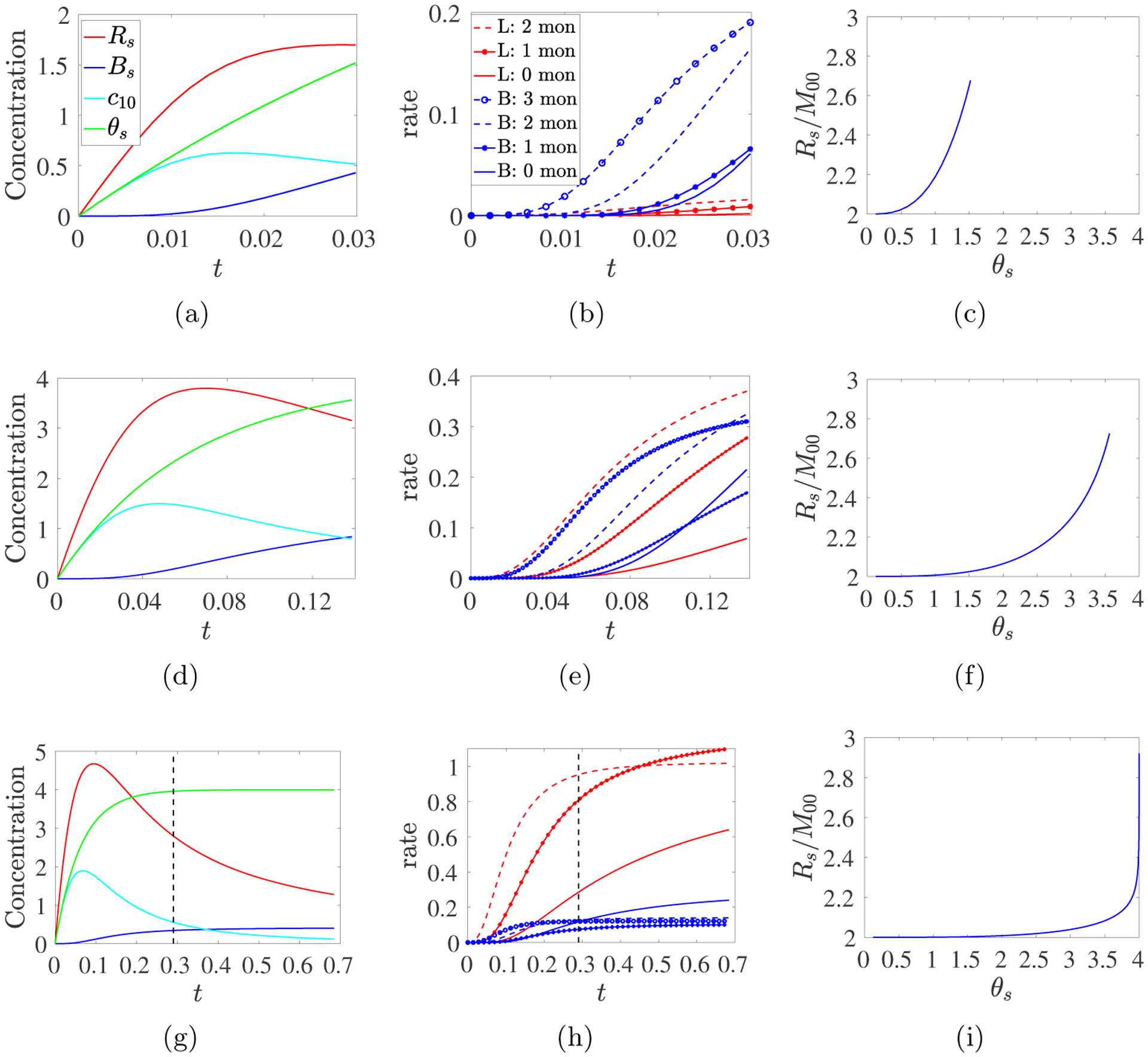
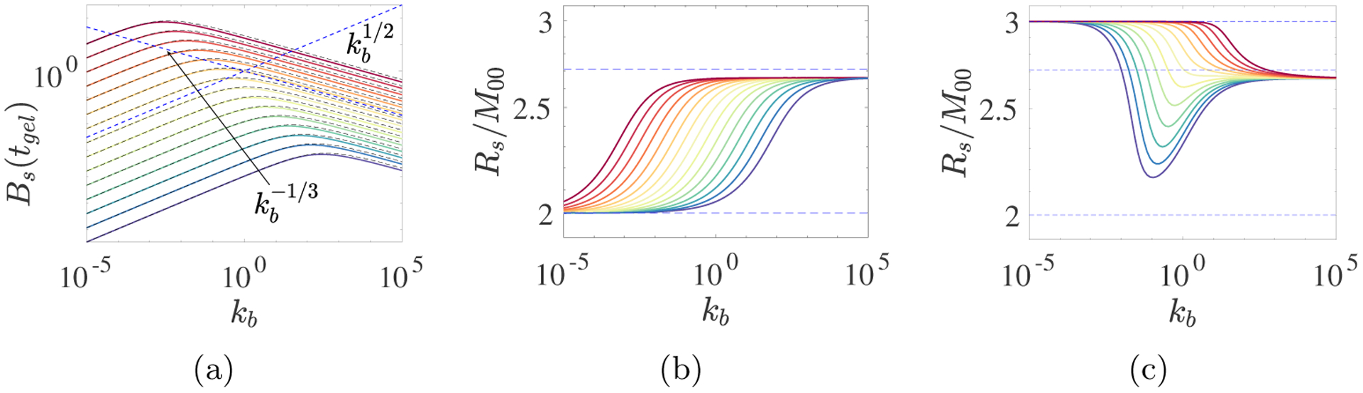
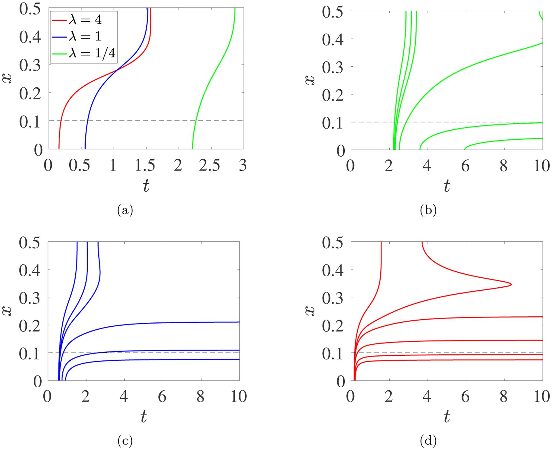
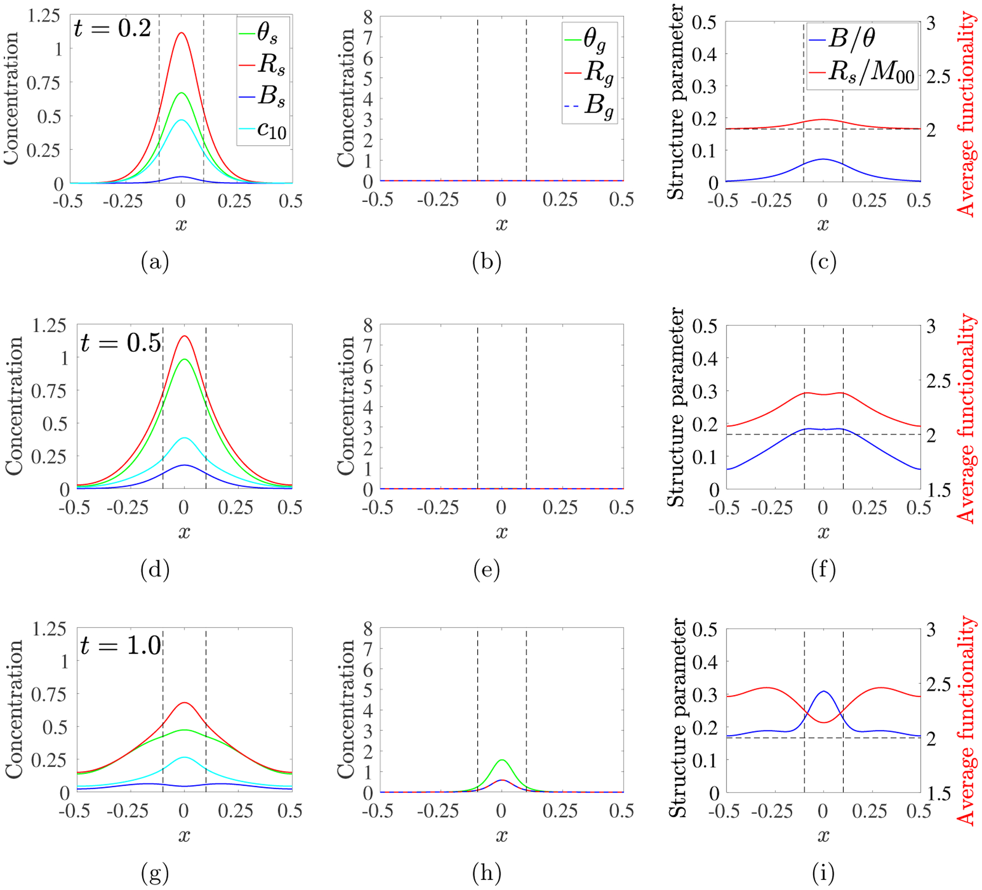
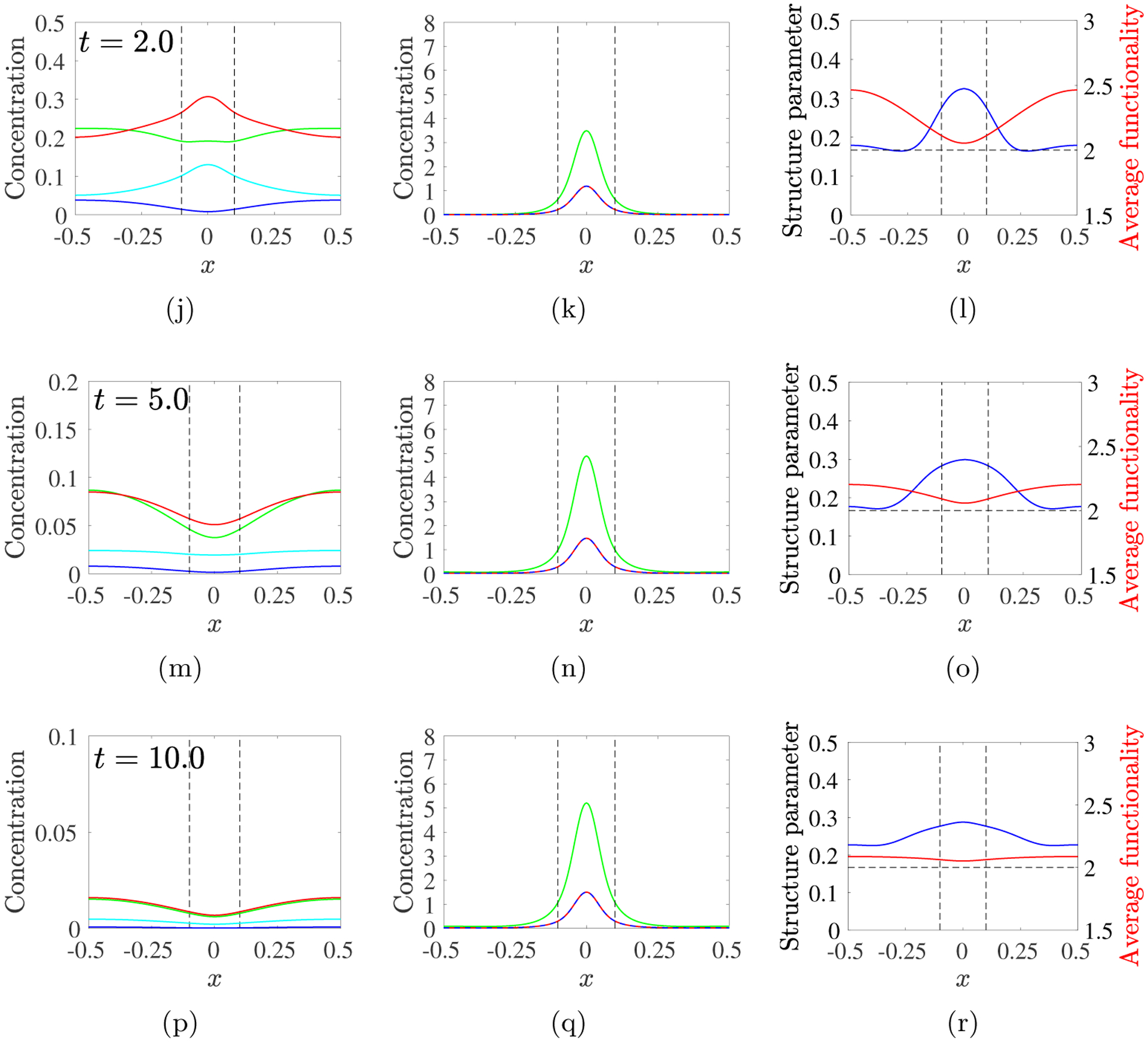
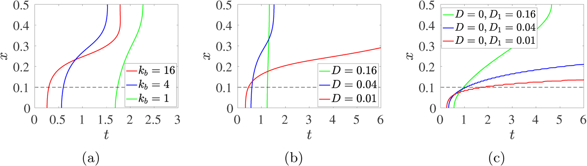
In [Fogelson and Keener, Phys. Rev. E, 81 (2010), 051922], we introduced a kinetic model of fibrin polymerization during blood clotting that captured salient experimental observations about how the gel branching structure depends on the conditions under which the polymerization occurs. Our analysis there used a moment-based approach that is valid only before the finite time blow-up that indicates formation of a gel. Here, we extend our analyses of the model to include both pre-gel and post-gel dynamics using the PDE-based framework we introduced in [Fogelson and Keener, SIAM J. Appl. Math., 75 (2015), pp. 1346-1368]. We also extend the model to include spatial heterogeneity and spatial transport processes. Studies of the behavior of the model reveal different spatial-temporal dynamics as the time scales of the key processes of branch formation, monomer introduction, and diffusion are varied.

Keywords: 82C26; 82D60; 92C05; 92C45; blood clotting; fibrin branching; gel front; generating function; kinetic gelation; polymer diffusion.

Fig. 1:

Schematic of fibrin polymerization showing thrombin-mediated fibrinopeptide release (top), protofibril formation (middle), and hypothesized [23] modes of branch formation (bottom).

Fig. 2:

(a) Linear polymerization to form a link. (b) Branch formation.

Fig. 3:

PDE Model with Spatially-uniform Initial Monomer Concentration: c₁₀(0) = 2, k_l = 1, k_b = 2. (a) Time snapshots of profiles W(t, z) vs z. The curves move upward with time and are colored red before gel time and blue afterward. Values of W(t, 1) for t > t_gel are shown with dots. (b) Plot of W(t, 1) vs t. Dots show (t, W(t, 1)) values corresponding to the dots in panel (a). (c) Time dependence of the concentrations of monomer c₁₀, sol reactive sites R_s, sol branches B_s, and mass in finite size oligomers larger than monomers θ_s − c₁₀. (d) Time dependence of the concentrations of gel reactive sites R_g, gel branches B_g, and gel mass θ_g. Note different concentration scales in panels (c) and (d). Dashed black line indicates gel time.

Fig. 4:

PDE Model with Spatially-uniform Monomer Source: c₁₀(0) = 0, S₁₀(t) = 0.25, k_l = 1, k_b = 10. Plots of c₁₀(t) (green), R_s(t) (red), B_s(t) (blue), θ_s(t) − c₁₀(t) (cyan), R_g(t) = B_g(t) (dashed red and blue) and θ_g(t) (dashed cyan).

Fig. 5:

Gillespie Simulations. Rate constants k_l = 1, k_b = 10, source rate S₁₀ = 0.25, and volume v = 10⁵. (a) Average oligomer size vs. t, (b) Largest oligomer size vs. t, (c) R(t), B(t), θ(t) and c₁₀(t) from Gillespie Simulation (colors) and ODE model (dashed black) show excellent agreement up to t_gel. (d) After t_gel, the mass density (θ_g), branch point density (B_g) and reaction site density (R_g) of the largest oligomer (colors) agree well with the corresponding gel variables (dashed black) from the PDE model.

Fig. 6:

PDE Model – Gel time as a function of m₀, λ, and k_b with the spatially-uniform time-varying monomer source S₁₀ = m₀λ exp(−λt). The heatmaps show log₁₀(t_gel) as a function of log₂(λ) and log₂(k_b). (a) m₀ = 2, (b) m₀ = 4, (c) m₀ = 8.

Fig. 7:

PDE model simulations with a spatially-uniform time-varying monomer source S₁₀ = m₀λ exp(−λt) for (a,d) m₀ = 2, (b,e) m₀ = 4, and (c,f) m₀ = 8. (a-c) Each curve corresponds to a specific λ value as indicated in the legend, and the points along each curve are for the different k_b values with the large dots indicating k_b = 1/8 and the k_b values increasing from that point to k_b = 32 at the other end of the curve. Note the different vertical scales. (d-f) The heatmaps show B_s(t_gel)/B_g(t_final).

Fig. 8:

PDE model simulations with a spatially-uniform time-varying monomer source S₁₀ = m₀λ exp(−λt) for (a) m₀ = 2, (b) m₀ = 4, and (c) m₀ = 8. Each curve corresponds to a specific λ value as indicated in the legend, and the points along each curve are for the different k_b values with the large dot indicating k_b = 1/8 and the k_b values increasing from that point to k_b = 32 at the other end of the curve.

Fig. 9:

ODE model simulations with a time-dependent source S₁₀(t) = m₀λ exp(−λt) with m₀ = 4 and λ = 16, and (abc) k_b = 32, (def) k_b = 1, (ghi) k_b = 1/8. (Left) Plots of R_s(t), B_s(t), c₁₀(t), and θ_s(t) until t = t_gel. (Middle) Rates of link and branching formation reactions involving different numbers of monomers. (Right) Average functionality f(t) = R_s(t)/M₀₀(t) vs. cumulative monomer sourced θ_s(t). Dashed black lines indicate when 99% of the monomer has been sourced.

Fig. 10:

ODE model calculations for various branching rates k_b and various (a,b) constant source rates S₁₀ and (c) time-varying source rates. (a) Colored curves show B_s(t_gel), blue dashed lines show its scaling behaviors, and black curves show approximate B_s(t_gel) from Eq. 3.10 using r_ss values computed by solving Eq. 3.5 numerically; (b) Colored curves show average functionality f^A = R_s/M₀₀ at t_gel. In (a) and (b), S₁₀ decreases from 10⁵ (deep red curve) to 10⁻⁵ (deep blue curve). Dashed blue line in (b) and (c) is 2/(1 − B_s/R_s) ≈ 2.7093 (see text). (c) Average functionality for time-varying source rate S₁₀(t) = m₀λ exp(−λt) m₀ = 4 and λ decreases from 10⁵ (deep red curve) to 10⁻⁵ (deep blue curve). Branching rates k_b vary as indicated.

Fig. 11:

PDE model simulations with source rate S₁₀(x, t) given in Eq. 3.12, with m₀ = 8, k_b = 4, λ = 0.25, 1.0, 4.0, contours of R_g in the xt–plane. (a) Contour R_g(x, t) = B_g(x, t) = 0.001 for λ = 4.0 (red), 1.0 (blue), and 0.25 (green). Each contour defines the gel front location x_gel(t) vs t. (b,c,d) Contours R_g(x, t) = B_g(x, t) = 0.001, 0.005, 0.01, 0.05, 0.25, and 0.50 (increasing from left to right) for (b) λ = 0.25, (c) λ = 1.0, and (d) λ = 4.0. The black dashed lines show the upper edge of the monomer source’s support. Note the different time interval in (a).

Fig. 12:

PDE model simulations with source rate S₁₀(x, t) given in Eq. 3.12, with m₀ = 8, k_b = 4, λ = 1, D = 0.04. Snapshots of sol variables (left) gel variables (middle), and structure variables (right) at the times indicated for each row. Note change in vertical scale in left column. Black dashed vertical lines show extent of source’s spatial support.

Fig. 12:

PDE model simulations with source rate S₁₀(x, t) given in Eq. 3.12, with m₀ = 8, k_b = 4, λ = 1, D = 0.04. Snapshots of sol variables (left) gel variables (middle), and structure variables (right) at the times indicated for each row. Note change in vertical scale in left column. Black dashed vertical lines show extent of source’s spatial support.

Fig. 13:

PDE model simulations with source rate S₁₀(x, t) given in Eq. 3.12, with m₀ = 8 and λ = 1 contours of R_g = 0.001 in the xt–plane for (a) D = 0.04 and k_b = 1, 4, 16, (b) k_b = 4 and D = 0.16, 0.04, 0.01, (c) k_b = 4, D = 0, and D₁ = 0.16, 0.04, 0.01, The black dashed lines show the upper edge of the monomer source’s support.

References

1. Blombäck B, Carlsson K, Fatah K, Hessel B, and Procyk R, Fibrin in human plasma: Gel architectures governed by rate and nature of fibrinogen activation, Thromb Res, 75 (1994), pp. 521–538. - PubMed
1. Campbell RA, Overmyer KA, Bagnell CR, and Wolberg AS, Cellular procoagulant activity dictates clot structure and stability as a function of distance from the cell surface, Arter Thromb Vasc Biol, 28 (2008), pp. 2247–2254. - PMC - PubMed
1. Campbell RA, Overmyer KA, Selzman CH, Sheridan BC, and Wolberg AS, Contributions of extravascular and intravascular cells to fibrin network formation, structure, and stability, Blood, 114 (2009), pp. 4886–4896. - PMC - PubMed
1. Chernysh IN, Nagaswami C, and Weisel JW, Visualization and identification of the structures formed during early stages of fibrin polymerization, Blood, 117 (2011), pp. 4609–4614. - PMC - PubMed
1. Chernysh IN and Weisel JW, Dynamic imaging of fibrin network formation correlated with other measures of polymerization, Blood, 111 (2008), pp. 4854–4861. - PMC - PubMed
LinkOut - more resources