Spatially resolved whole transcriptome profiling in human and mouse tissue using Digital Spatial Profiling

Abstract

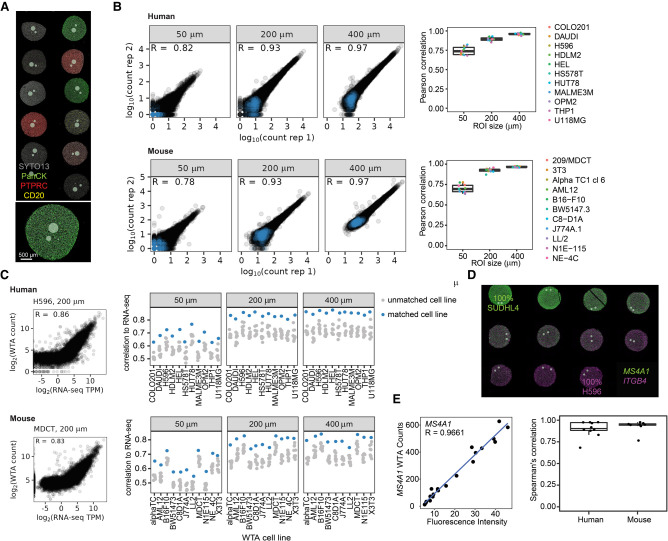
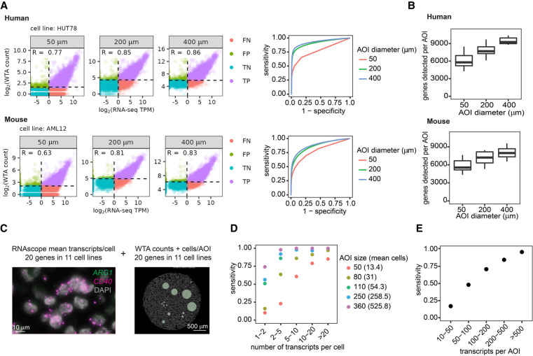
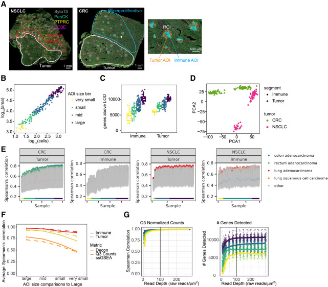
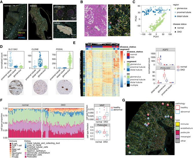
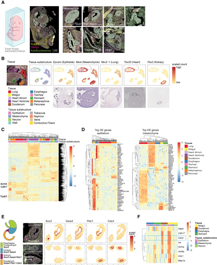
Emerging spatial profiling technology has enabled high-plex molecular profiling in biological tissues, preserving the spatial and morphological context of gene expression. Here, we describe expanding the chemistry for the Digital Spatial Profiling platform to quantify whole transcriptomes in human and mouse tissues using a wide range of spatial profiling strategies and sample types. We designed multiplexed in situ hybridization probes targeting the protein-coding genes of the human and mouse transcriptomes, referred to as the human or mouse Whole Transcriptome Atlas (WTA). Human and mouse WTAs were validated in cell lines for concordance with orthogonal gene expression profiling methods in regions ranging from ∼10-500 cells. By benchmarking against bulk RNA-seq and fluorescence in situ hybridization, we show robust transcript detection down to ∼100 transcripts per region. To assess the performance of WTA across tissue and sample types, we applied WTA to biological questions in cancer, molecular pathology, and developmental biology. Spatial profiling with WTA detected expected gene expression differences between tumor and tumor microenvironment, identified disease-specific gene expression heterogeneity in histological structures of the human kidney, and comprehensively mapped transcriptional programs in anatomical substructures of nine organs in the developing mouse embryo. Digital Spatial Profiling technology with the WTA assays provides a flexible method for spatial whole transcriptome profiling applicable to diverse tissue types and biological contexts.

Figure 1.

Human and mouse WTA data are reproducible and correlated with RNA-seq and RNA FISH. (A) Representative image of the areas of illumination (AOI)-size titration experiment. Circular AOIs 50 μm, 200 μm, and 400 μm in diameter were placed on each cell line of an 11-core human or mouse formalin-fixed paraffin embedded (FFPE) cell pellet array (human shown, stained with antibodies against CD3E, PTPRC, and pan-cytokeratin [PanCK], and SYTO13 nuclear stain). (B) Reproducibility of WTA counts from two replicate experiments. Left: Scatterplots of log₁₀-transformed raw counts from one representative human (HUT78) or mouse (3T3) cell line at each AOI size from each replicate. Negative control probes are shown in blue and target probes in black. Right: Pearson correlation coefficients of log₁₀-transformed raw counts between replicates for each cell line and AOI size. (C) Left: Scatterplots of WTA counts versus RNA-seq TPM from the same cell line for one representative human or mouse cell line in a 200 μm AOI. Right: Spearman's correlation of WTA counts compared with RNA-seq of each cell line. For each AOI, the matching cell line is shown in blue and all other cell lines in gray. (D) Representative image of the cell line titration experiment. Cell pellets contained one cell line titrated into the other at a variable ratio. Cells were stained with RNAscope probes against two genes specifically expressed in one of the two cell lines. Gray circles show profiled AOIs. (E) Left: Representative scatterplot comparing WTA counts for MS4A1 to RNAscope fluorescence intensity for the same gene across cell pellets. Right: Spearman's correlation of WTA counts compared with RNA FISH fluorescence intensity for each gene profiled.

Figure 2.

WTA has high sensitivity and can detect genes at a range of expression levels depending on areas of illumination (AOI) size. (A) Left: Scatterplots comparing WTA counts to RNA-seq for one representative cell line at each AOI size, colored by whether the gene is detected above the expression threshold in each assay. Dashed lines indicate thresholds for calling a gene “expressed” as 2 standard deviations above the geometric mean of negative probes for WTA, and TPM > 1 for RNA-seq. TP, true positive; FP, false positive; TN, true negative; and FN, false negative. Right: Receiver-operator curves demonstrating the sensitivity and specificity of WTA at different WTA expression thresholds. (B) Number of genes per AOI above the expression threshold of 2 standard deviations above the mean negative probe count at each AOI size. (C) Representative images of the experiment to determine the sensitivity of human WTA relative to absolute transcript number. Left: RNAscope image of two genes in one cell line of the 20 genes in 11 cell lines quantified in this experiment. Right: Digital Spatial Profiling (DSP) image of one cell line with an AOI size titration. (D) Sensitivity of WTA at different AOI sizes for genes in different gene expression bins as measured by RNAscope. Genes ≥ 1 transcript per cell were considered expressed. Intervals are open on the left and closed on the right. (E) Sensitivity of WTA for genes binned by transcripts per AOI, calculated using transcripts per cell quantified by RNAscope and the number of cells in each AOI.

Figure 3.

Effect of areas of illumination (AOI) size and sequencing depth on biological conclusions from segmented tumor and tumor microenvironment. (A) Left: Representative images of the colorectal cancer (CRC) and non-small cell lung cancer (NSCLC) samples. Tumor, invasive-margin, and hyperproliferative regions are highlighted. Tissues were stained with antibodies against PanCK, CD3E, and PTPRC. Right: Enlarged region of the CRC image to highlight the size titration and segmentation strategy. Circular regions of interest were automatically segmented into tumor (orange) and immune (blue) compartments. (B) Scatterplot of AOI area versus number of cells with points colored by area bin: Very small, <2300 μm²; small, 2300–7850 μm²; mid, 7850–49,000 μm²; large, >49,000 μm². (C) Number of genes detected per AOI for tumor and immune compartments in each AOI size bin, colored as in B. (D) Principal component analysis of variation between samples using genes detected above background in >20% of AOIs. PC1 versus PC2 is plotted with points colored by tumor type and shaped by segment type. (E) Spearman's correlation of WTA counts from each AOI with all RNA-seq data sets in TCGA. AOIs are ordered by area on the x-axis, and each point is a pairwise comparison with a data set in TCGA. Points are colored by TCGA tumor type: colon adenocarcinoma (blue), rectal adenocarcinoma (green), lung adenocarcinoma (red), lung squamous cell carcinoma (orange), and other (gray). AOIs are labeled by area bin, colored as in B. (F) Correlation of counts, single-sample Gene Set Enrichment Analysis (ssGSEA) enrichment, and cell type deconvolution between AOIs. For each metric, Spearman's correlations were calculated between each AOI compared with the largest AOI sizes, and averaged within different AOI size bins. (G) Left: Spearman's correlation of counts for each subsampled read depth and AOI size relative to counts at 300 reads/μm². Right: Number of genes detected above background for each read depth and AOI size.

Figure 4.

Spatial heterogeneity in gene expression changes associated with diabetic kidney disease in human kidneys. (A) Left: Representative fluorescence images of normal and diabetic human kidneys. Tissues were stained with antibodies against PanCK, WT1, and PTPRC. Right: Example images from a normal kidney highlighting the AOI strategy. Glomeruli were profiled using polygon-shaped areas of illuminations (AOIs), and tubules were automatically segmented into proximal tubules (PanCK⁻) and distal tubules (PanCK⁺). (B) Individual glomeruli in each kidney sample were annotated by degree of pathology. A representative H&E image (left) and fluorescence image (right) from the same region of a diabetic kidney disease (DKD) specimen are shown. Glomeruli with a higher degree of abnormality are circled in gray and labeled “A”, whereas more normal glomeruli are circled in white and labeled “N”. (C) Principal component analysis of variation between samples using genes detected above background in >1% of AOIs. PC1 versus PC2 is plotted, with substructure indicated by color and disease status indicated by shape. (D) Boxplots of counts in all AOIs of three example genes differentially expressed between kidney substructures with the corresponding antibody-stained images from the Human Protein Atlas (https://www.proteinatlas.org/) (Uhlén et al. 2015). (E) Left: Heatmap of differentially expressed genes between normal and DKD in glomeruli, distal tubules, and proximal tubules. All genes are significant at FDR < 0.05 and a fold change of >1.5. Genes are annotated by the structure in which they were significantly differentially expressed, or “multiple” for the genes significant in more than one structure. Columns and rows are clustered by hierarchical clustering and the data are scaled by row. Right: Boxplot of normalized counts for two example differentially expressed genes in normal and DKD kidney structures. (F) Left: Results of cell type deconvolution of glomeruli using single-cell expression data from Young et al. (2018). Data are displayed as stacked barplots with each bar as a single AOI and the estimated proportion of each cell type colored, faceted by disease status. Right: Boxplots of proportions of two example differentially abundant cell types in normal and DKD glomeruli (t-test Bonferroni-corrected P-value < 0.05). MNP, mononuclear phagocytes; DC, dendritic cells. (G) Pie charts overlaid on the fluorescence image of a single kidney, showing the proportion of different glomerulus and immune cell types for each glomerulus profiled in a representative disease sample. Each plot is outlined based on pathological annotation: abnormal glomeruli (blue), healthy glomeruli (red).

Figure 5.

Spatial profiling of transcriptional programs during organogenesis in a midgestation mouse embryo. (A) Left: Schematic and representative image of the fixed frozen E13.5 mouse embryo profiled. Embryos were labeled with antibodies against TRP63 (magenta) and TUBB3 (yellow). Autofluorescence is shown in green. Right: Example images of each organ profiled showing the areas of illumination (AOI) profiling strategy. Freeform polygon AOIs capture anatomical substructures of each organ. (B) Expression of marker genes for specific organs and cell types in an example section compared with in situ hybridization (ISH) images of the same genes in E14.5 mouse embryos from the GenePaint database (https://gp3.mpg.de/, Diez-Roux et al. 2011; Visel et al. 2004). Tissue, tissue substructure, or normalized scaled WTA count is plotted over the shape of each AOI. (C) Heatmap showing scaled expression of the 2000 most variable genes across the data set. Columns and rows are clustered by hierarchical clustering and columns are annotated by organ and organ substructure. (D) Heatmaps showing scaled expression of the top 50 most differentially expressed genes in epithelium (left) and mesenchyme (right). All genes shown are significant at Bonferroni-corrected P-value < 0.01. Columns and rows are clustered by hierarchical clustering and columns are annotated by organ. (E) Left: Schematic of key transcription factor expression in stomach and gut development (adapted from Willet and Mills 2016). Right: Expression of the same transcription factors plotted on example AOIs from a representative section. (F) Heatmap showing scaled expression of Cdx2 and Cdx2-target genes from Gao et al. (2009) in esophagus, stomach, duodenum, and midgut AOIs. Columns and rows are clustered by hierarchical clustering and columns are annotated by organ and organ substructure.

References

1. Aigha II, Abdelalim EM. 2020. NKX6.1 transcription factor: a crucial regulator of pancreatic β cell development, identity, and proliferation. Stem Cell Res Ther 11: 459. 10.1186/s13287-020-01977-0 - DOI - PMC - PubMed
1. Bergholtz H, Carter JM, Cesano A, Cheang MCU, Church SE, Divakar P, Fuhrman CA, Goel S, Gong J, Guerriero JL, et al. 2021. Best practices for spatial profiling for breast cancer research with the GeoMx® Digital Spatial Profiler. Cancers (Basel) 13: 4456. 10.3390/cancers13174456 - DOI - PMC - PubMed
1. Bouchard M, Souabni A, Mandler M, Neubüser A, Busslinger M. 2002. Nephric lineage specification by Pax2 and Pax8. Genes Dev 16: 2958–2970. 10.1101/gad.240102 - DOI - PMC - PubMed
1. Brady L, Kriner M, Coleman I, Morrissey C, Roudier M, True LD, Gulati R, Plymate SR, Zhou Z, Birditt B, et al. 2021. Inter- and intra-tumor heterogeneity of metastatic prostate cancer determined by digital spatial gene expression profiling. Nat Commun 12: 1426. 10.1038/s41467-021-21615-4 - DOI - PMC - PubMed
1. Breschi A, Gingeras TR, Guigó R. 2017. Comparative transcriptomics in human and mouse. Nat Rev Genet 18: 425–440. 10.1038/nrg.2017.19 - DOI - PMC - PubMed