Inferring structural and dynamical properties of gene networks from data with deep learning

Abstract

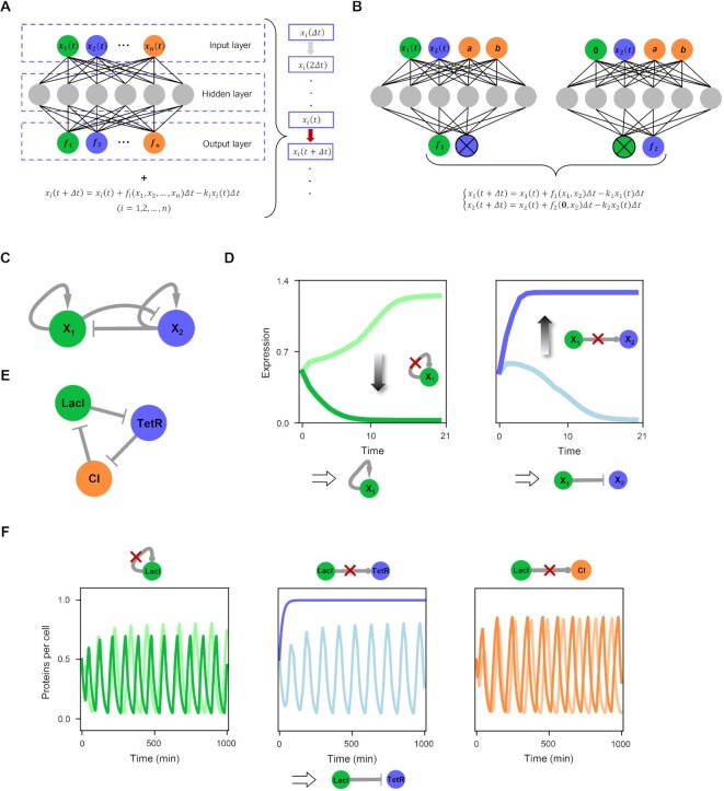
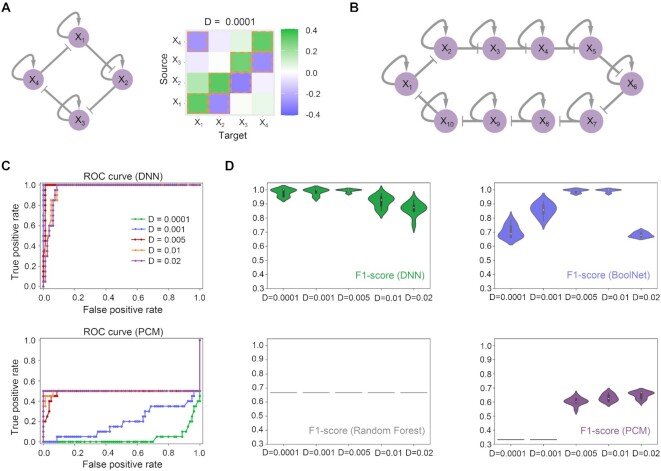
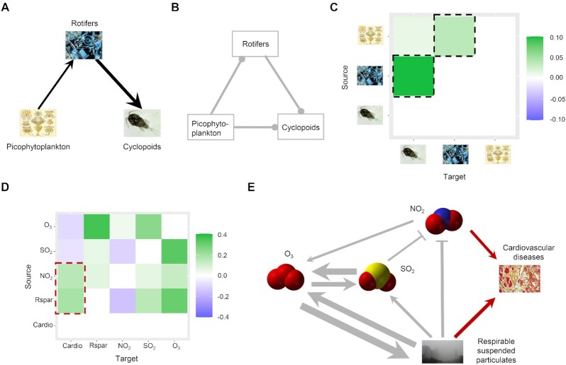
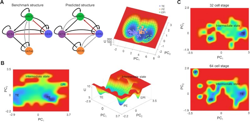
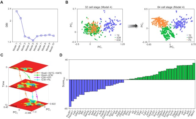
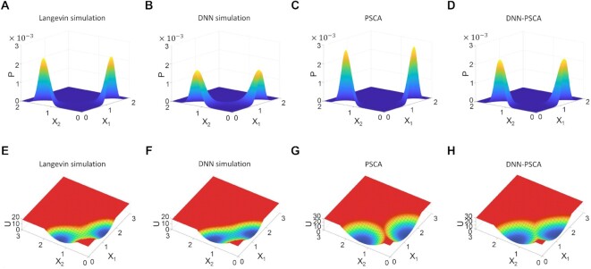
The reconstruction of gene regulatory networks (GRNs) from data is vital in systems biology. Although different approaches have been proposed to infer causality from data, some challenges remain, such as how to accurately infer the direction and type of interactions, how to deal with complex network involving multiple feedbacks, as well as how to infer causality between variables from real-world data, especially single cell data. Here, we tackle these problems by deep neural networks (DNNs). The underlying regulatory network for different systems (gene regulations, ecology, diseases, development) can be successfully reconstructed from trained DNN models. We show that DNN is superior to existing approaches including Boolean network, Random Forest and partial cross mapping for network inference. Further, by interrogating the ensemble DNN model trained from single cell data from dynamical system perspective, we are able to unravel complex cell fate dynamics during preimplantation development. We also propose a data-driven approach to quantify the energy landscape for gene regulatory systems, by combining DNN with the partial self-consistent mean field approximation (PSCA) approach. We anticipate the proposed method can be applied to other fields to decipher the underlying dynamical mechanisms of systems from data.

Figure 1.

General DNN framework and its application on MISA model and oscillation system. (A) The deep neural network framework. The input is the gene expression of X_i(i = i, 2, ..., n) at time t, the output is f_i, and then the formula is used to calculate the gene expression of X_i at time t + Δt. In this loop, x_i(t + Δt) is introduced into the model to obtain x_i(t + 2Δt). (B) The edge removal strategy for the reconstruction of network structure. Setting the gene expression level of X₁ to zero will eliminate the direct regulation of gene X₁ on gene X₂. (C) The structure diagram of the MISA model. The green and blue round dots indicate genes, the arrows indicate positive regulation, and the blunt arrows indicate negative regulation. Here, genes X₁ and X₂ are symmetrical, activating themselves and inhibiting each other. (D) Reconstruction of the network structure when the diffusion constant is 0.0004. The parameters are set as a = 0.5, b = 0.8. In this case the system has two stable states. The dark blue (green) and light blue (green) lines indicate the trajectory of gene X₂ (X₁) after and before edge removal, individually. (E) The oscillation network for repressilator. The oscillation network is a cyclic negative-feedback loop composed of three genes. (F) Inference of the interaction regarding gene LacI in the oscillation network. If we delete a non-existent interaction (for example, the regulation of LacI on CI), the target variable (CI) still maintains oscillation, while if we remove an existing interaction (the regulation of LacI on TetR), the target variable (TetR) no longer exhibits an oscillation pattern.

Figure 2.

The comparison of different methods for network inference. (A) Structure diagram of the four-dimensional gene network system, and the prediction result of DNN for network inference under the noise level D = 0.0001 (right panel), where the vertical axis represents the source of regulation, and the horizontal axis represents the target of regulation. Here, green boxes (blue) indicate positive (negative) regulations and the darker (lighter) the color, the stronger (weaker) the regulation is. The yellow boxes represent the predicted interaction, which are fully consistent with the network structure on the left. (B) Structure diagram of the 10D gene network system. (C) ROC curves of DNN and PCM at different noise levels. (D) F1-score statistics of DNN, BoolNet, Random Forest and PCM under different noise levels (10 trials, the data set used by each trial contains 3600 time series).

Figure 3.

Reconstructing networks from real-world data. (A) A food chain network composed of three types of plankton, where the thickness of the arrows represents the food preferences of the species and the direction of each black arrow represents the interaction between prey and predator. (B) The prior structure used in DNN. Arrows ending with a dot characterize the interaction with directions but without the interaction type. (C) The interaction predicted by DNN, where the square marked by the black box are consistent with the black arrow in (A). (D) The results of all interactions between air pollutants and cardiovascular diseases predicted by DNN. (E) The reconstructed network based on (D), where the thickness of the arrow indicates the intensity of interaction. The red arrows highlight the causal interactions on cardiovascular diseases, which correspond to the red boxes in (D).

Figure 4.

Inference of structure and energy landscape from single cell date. (A) The reconstruction of a small-scale gene networks from single-cell data. The left panel is the benchmark structure, and the middle panel is the structure predicted by the DNN. Black arrows denote the consistent interaction of the two structures, red arrows denote the links in the same direction but different type. The right panel shows the validation of the predicted structure, as its corresponding Hill function model closely matches the single cell data, where the landscape is derived from the corresponding Hill function model, and the points are single cell data. (B) The two-dimensional and three-dimensional energy landscape for the 48-dimensional model of mouse development constructed from single-cell data (all stages) via DNN. Four attractors (characterizing cell types) including EPI, TE, PE and intermediate state emerge on the landscape. (C) The two-dimensional landscapes at 32-cell and 64-cell stage modeled by DNN.

Figure 5.

DNN model identifies the lineage transition path and critical genes for cell fate transitions. (A) The DBI value for three clusters for different models. Here, model 1 is for k = 0.05, model 2 is an ensemble model for k = 0.05 and k = 0.15, and so on. (B) The cell clusters for 32-cell and 64-cell stage in reduced PC dimensions from model 4. It can be seen that the ICM cells in stage 32 (left panel) differentiate into EPI cells and PE cells in 64-cell stage (right panel), respectively. (C) Landscape at 16, 32 and 64-cell stage and corresponding transition paths predicted by model 4. Each path is the average of thousands of corresponding trajectories. (D) Score_DBI with different genes knocked out. A negative Score_DBI indicates that the simulated 64-cell stage data after gene knockout tend to be divided into two clusters. Since cells in 64-cell stage should be divided into three clusters in wild-type, namely PE, TE and EPI, it means that knocking out corresponding gene result in the loss of cell clusters.

Figure 6.

Comparisons among different methods for calculating probability distributions and corresponding energy landscapes. (A–D) The distribution calculated by Langevin simulation, DNN simulation, PSCA and DNN-PSCA. (E–H) The potential landscapes corresponding to (A–D). The distribution calculated from PSCA based on the explicit model is closest to that from Langevin simulation (, d_KL = 0.1121), followed by DNN-PSCA (, d_KL = 0.1426) and DNN simulation (, d_KL = 0.2871).

References

1. Li C., Wang J.. Quantifying cell fate decisions for differentiation and reprogramming of a human stem cell network: landscape and biological paths. PLoS Comput. Biol. 2013; 9:e1003165. - PMC - PubMed
1. MacArthur B.D., Ma’ayan A., Lemischka I.R.. Systems biology of stem cell fate and cellular reprogramming. Nat. Rev. Mol. Cell Biol. 2009; 10:672–681. - PMC - PubMed
1. Collombet S., van Oevelen C., Sardina Ortega J.L., Abou-Jaoudé W., Di Stefano B., Thomas-Chollier M., Graf T., Thieffry D.. Logical modeling of lymphoid and myeloid cell specification and transdifferentiation. Proc. Natl. Acad. Sci. U.S.A. 2017; 114:5792–5799. - PMC - PubMed
1. Zhang B., Wolynes P.G.. Stem cell differentiation as a many-body problem. Proc. Natl. Acad. Sci. U.S.A. 2014; 111:10185–10190. - PMC - PubMed
1. Lin Y.T., Hufton P.G., Lee E.J., Potoyan D.A.. A stochastic and dynamical view of pluripotency in mouse embryonic stem cells. PLoS Comput. Biol. 2018; 14:e1006000. - PMC - PubMed