Local stressors mask the effects of warming in freshwater ecosystems

Abstract

Climate warming is a ubiquitous stressor in freshwater ecosystems, yet its interactive effects with other stressors are poorly understood. We address this knowledge gap by testing the ability of three contrasting null models to predict the joint impacts of warming and a range of other aquatic stressors using a new database of 296 experimental combinations. Despite concerns that stressors will interact to cause synergisms, we found that net impacts were usually best explained by the effect of the stronger stressor alone (the dominance null model), especially if this stressor was a local disturbance associated with human land use. Prediction accuracy depended on stressor identity and how asymmetric stressors were in the magnitude of their effects. These findings suggest we can effectively predict the impacts of multiple stressors by focusing on the stronger stressor, as habitat alteration, nutrients and contamination often override the biological consequences of higher temperatures in freshwater ecosystems.

Keywords: antagonisms; aquatic ecology; dominance null model; global change; multiple stressors; stressor interactions.

FIGURE 1

Examples of predicted responses from the multiplicative, additive and dominance models when stressor pairs (S_A = stressor a, S_B = stressor B) have positive (a), contrasting (b) or negative (c) effects relative to the control, which varies in the different scenarios (ABS = absolute). Responses include plant or animal survival, growth/size, condition, biomass, abundance, diversity and decomposition measured from experimental treatments. An overview of our empirical results (d) shows the best performing null models across all (296) responses and the percentage of observations that fell within or beyond the range predicted by all three null models. Undefined responses are those where multiple null models were indistinguishable in their performance.

FIGURE 2

Percentage of observed responses to warming paired with another stressor that fall within or beyond the range predicted by all three null models grouped by stressor type (a) and organisation level (b) for the entire dataset (n = 296). Directions are on an absolute scale (e.g. observed responses larger than predicted were either more negative or more positive).

FIGURE 3

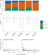
Asymmetric stressors. Frequency of responses best predicted by additive (blue), dominance (orange) and multiplicative (green) models (a) and their mean effect sizes (Hedges' d) showing standardised differences between observed effects and those predicted for each null model (with 95% confidence intervals; (b) across types of secondary stressors combined with temperature, when stressors were not strongly asymmetric or when either temperature, habitat alteration, nutrient levels or contamination had prevailing independent effects (effect >50% higher than the other). Mean effect sizes of zero indicate no difference between observed responses ($X_o$) and null model predictions ($X_p$). Mean observed effects are considered statistically indistinguishable from null model predictions when confidence intervals cross zero. Significant negative effect sizes indicate that observed responses were smaller (antagonistic; either less negative or less positive) than predicted. Although not seen here, significant positive effect sizes would indicate that observed responses were larger (more negative or more positive) than predicted. Panel (c) shows the absolute effect size for each null model with increasing asymmetry (% difference in independent effects) where either temperature or the second stressor are the prevailing independent stressor fitted with GLMs. Increasing (decreasing) absolute effect sizes indicate increasing (decreasing) deviation from null model predictions.

FIGURE 4

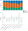
Stressor pairs. Frequency of responses best predicted by additive (blue), dominance (orange) and multiplicative (green) models (a) and mean effect sizes (Hedges' d) showing standardised differences between observed effects and those predicted for each null model (with 95% confidence intervals; (b) across types of secondary stressors combined with temperature, T. mean effect sizes of zero indicate no difference between observed responses ($X_o$) and null model predictions ($X_p$). Mean observed effects are considered statistically indistinguishable from null model predictions when confidence intervals cross zero. Significant negative effect sizes indicate that observed responses were smaller (either less negative or less positive) than null model predictions. Although not seen here, significant positive effect sizes would indicate that observed responses were larger (more negative or more positive) than predicted. Samples sizes may differ from Figure 1 because outliers were removed from mean effect calculations (see Methods).

FIGURE 5

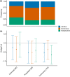
Biological organisation. Frequency of responses best predicted by additive (blue), dominance (orange) and multiplicative (green) models (a) and their mean effect sizes (Hedges' d) showing standardised differences between observed effects and those predicted for each null model (with 95% confidence intervals; (b) across levels of biological organisation. Mean effect sizes of zero indicate no difference between observed responses ($X_o$) and null model predictions ($X_p$). Mean observed effects are considered statistically indistinguishable from null model predictions when confidence intervals cross zero. Significant negative effect sizes indicate that observed responses were smaller (either less negative or less positive) than null model predictions. Although not seen here, significant positive effect sizes would indicate that observed responses were larger (more negative or more positive) than predicted.

References

1. Ban, S.S. , Graham, N.A.J. & Connolly, S.R. (2014) Evidence for multiple stressor interactions and effects on coral reefs. Global Change Biology, 20, 681–697. - PubMed
1. Bancroft, B.A. , Baker, N.J. & Blaustein, A.R. (2008) A meta‐analysis of the effects of ultraviolet B radiation and its synergistic interactions with pH, contaminants, and disease on amphibian survival. Conservation Biology, 22, 987–996. - PubMed
1. Birk, S. , Chapman, D. , Carvalho, L. , Spears, B.M. , Andersen, H.E. , Argillier, C. et al. (2020) Impacts of multiple stressors on freshwater biota across spatial scales and ecosystems. Nature Ecology & Evolution, 4(8), 1060–1068. - PubMed
1. Boyd, P.W. , Collins, S. , Dupont, S. , Fabricius, K. , Gattuso, J.‐P. , Havenhand, J. et al. (2018) Experimental strategies to assess the biological ramifications of multiple drivers of global ocean change—a review. Global Change Biology, 24, 2239–2261. - PubMed
1. Brooks, P.R. & Crowe, T.P. (2018) Density and biotic interactions modify the combined effects of global and local stressors. Oikos, 127, 1746–1758.
LinkOut - more resources