Predicting fertility from sperm motility landscapes

Abstract

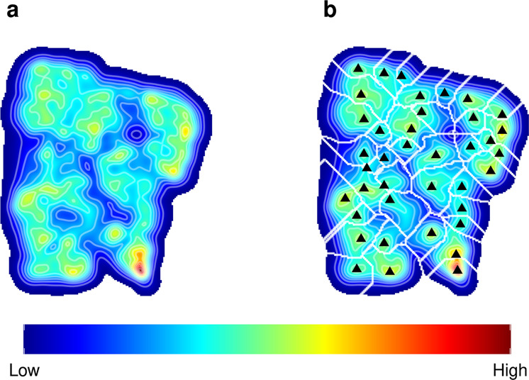
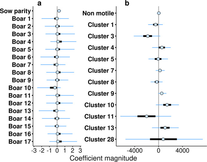
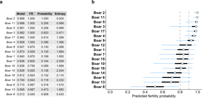
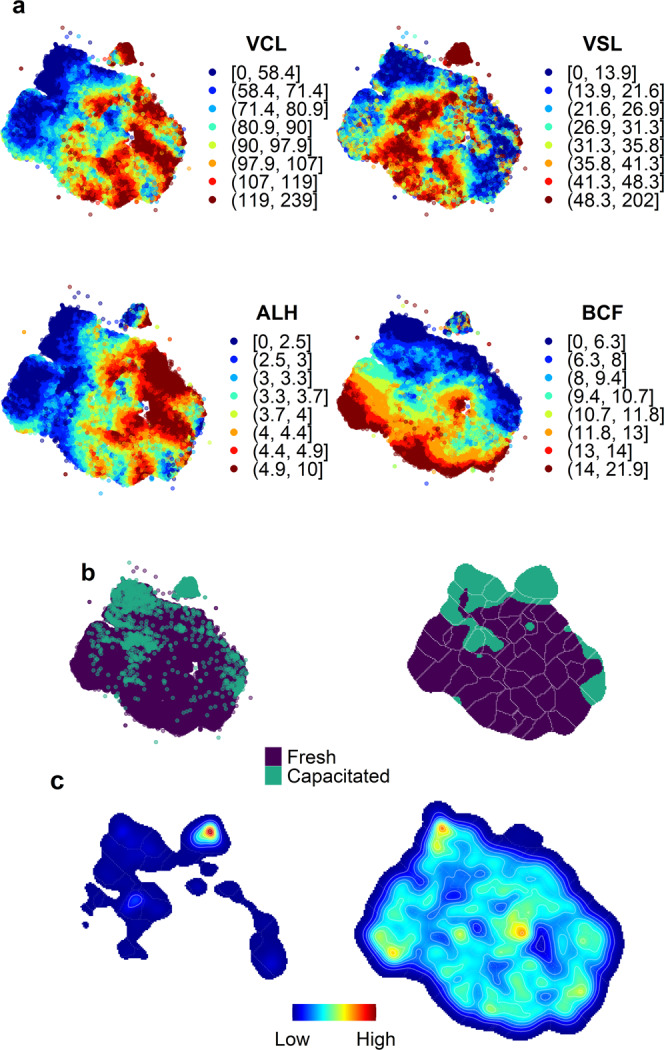
Understanding the organisational principles of sperm motility has both evolutionary and applied impact. The emergence of computer aided systems in this field came with the promise of automated quantification and classification, potentially improving our understanding of the determinants of reproductive success. Yet, nowadays the relationship between sperm variability and fertility remains unclear. Here, we characterize pig sperm motility using t-SNE, an embedding method adequate to study behavioural variability. T-SNE reveals a hierarchical organization of sperm motility across ejaculates and individuals, enabling accurate fertility predictions by means of Bayesian logistic regression. Our results show that sperm motility features, like high-speed and straight-lined motion, correlate positively with fertility and are more relevant than other sources of variability. We propose the combined use of embedding methods with Bayesian inference frameworks in order to achieve a better understanding of the relationship between fertility and sperm motility in animals, including humans.

Fig. 1. Sperm motility landscape resulting from a (Barnes-Hut approximation) t-SNE dimensional reduction.

a Kernel density showing the high- and low-density regions within the landscape, computed in a 200 × 200 cell grid with a neighbouring parameter representing a 1% of the dataset size (perplexity = 639). b Clustering using a watershed algorithm allowing the discretization of data into clusters (delimited by the white lines), and depicting the highest density peak within each cluster (black triangles). The legend describes the colour gradient in the density kernel. This analysis involves functions "bdm.pakde" and "bdm.wtt" in the bigMap R package. See also "Sperm motility landscape" in Methods and Garriga & Bartumeus 2018).

Fig. 2. Estimates of the coefficients and their uncertainty in the fertility model.

The medians of the coefficients are depicted with a clear point, thick black bars represent the 50% credible intervals (C.I.), and the thin lines represent 95% C.I. a Coefficients of animal-related factors (sow parity, individual boars). Sow parity corresponds to the number of times that the sow completed a cycle of insemination. The boars (from 1 to 17) are intercepts that vary amongst individuals (usually known as random effect). b Coefficients corresponding to sperm behaviour related factors (the proportion of non-motile sperm, and the relative proportions of sperm in each of the motility clusters represented in the landscape). Note the different values in the x-axis (coefficient magnitude) for a, b.

Fig. 3. Impact of sperm motility features on fertility.

a Boxplots of the motility features (VCL, curvilinear velocity; VSL, straight-line velocity; ALH lateral amplitude of head displacement; BCF, beat-cross frequency; VAP, average path velocity; LIN, linearity; STR, straightness; and WOB, wobble) grouped by their effect (either positive or negative) on fertility, according to model M3. Mean values (positive-negative) for each motility variable: ALH (3.94−3.26 μm), VAP (48.72−40.29 μm/s), STR (71.61−54.26%), LIN (39.60−28.49%), VSL (34.94−23.64 μm/s), BCF (10.03−10.14 Hz), WOB (54.50−48.52%) and VCL (90.80−79.19 μm/s). Mean comparisons between the two groups (two-sided unpaired T-student tests; number of samples per group: positive = 36482, negative = 32688) yielded a p value < 10⁻¹⁵ in all motility variables, except for BCF (p value < 10⁻³). Both groups met the assumptions of T-student test in all variables tested. b 11-cluster motility landscape showing the clusters with positive (light green) and negative (dark green) correlation with fertility, according to model M3. The high-density peaks (labelled with the cluster number) are also depicted, as well as contour lines to help visualise the stereotypes (as in Fig. 1).

Fig. 4. Predicted fertility per boar.

The values represent the median predicted fertility, expressed as probability of success (successful oocyte fertilisation). a Table of comparison between the estimated (posterior median) fertility, and the farrowing rate (FR), a commonly used measure of fertility. The boars are ranked in descending order according to the predictions of the model. The pseudo-probability (in a 1000 iteration bootstrap) is presented for each boar to be ranked in the current position. Additionally, entropy (calculated as $-{\sum }_{i=1}^{17}{p}_{i}ln\left(p_i\right)$, where p is the probability of belonging to ith position) is used as a measure of position diversity for each of the boars. Namely, a higher entropy corresponds to boars that can be found in a broader range of positions, whereas a lower entropy corresponds to more robust boars. The Kendall’s correlation between the predicted rank and the FR rank was calculated at each bootstrap iteration, yielding a mean correlation of 0.826 ± 0.055 (ranging from 0.662 to 1.000), with a mean p value of 1.7 × 10⁻⁶ ± 6.2 × 10⁻⁶ (ranging from 5.5 × 10⁻¹⁵ to 8.2 × 10⁻⁵). b Predictions with their corresponding uncertainty around the median (open dot). 50% credible intervals (C.I.) are represented by thick, black lines, while 95% C.I. are represented with blue thin lines. Boars are sorted in descending order, according to their estimated fertility (median). The vertical dotted lines represent thresholds at 0.8 and 0.9, corresponding with the categorisation of boars (relatively low or high fertility, respectively).

Fig. 5. Sperm motility features of fresh and capacitated sperm.

a Quantile map of the motility features used in the t-SNE (VCL curvilinear velocity, VSL straight-line velocity, ALH lateral amplitude of the head displacement, and BCF beat-cross frequency). Colours represent an interval of values (eight percentiles, from 0–12.5 to 87.5–100) of each variable amended for a gradient visualisation. b Location of fresh sperm (purple) and capacitated sperm (green). Sperm labelled as capacitated were kept in a medium that elicits in vitro capacitation (containing albumin, bicarbonate and calcium, amongst others). The left panel is a pointwise representation of capacitated and fresh sperm. The right panel depicts a cell-wise hard clustering in a 200 × 200 grid. Cells were assigned "capacitated" or "fresh" depending on the density of points in each category (i.e., if a cell had a higher proportion of fresh sperm, it was labelled as fresh, and capacitated otherwise). c Heatmap of the landscape distribution of capacitated (left panel) and fresh sperm (right panel).

Fig. 6. Model selection based on sperm motility landscape configurations.

a Signal-to noise ratio (S2NR) as an heuristic of information gain, along the process of merging. The information generally increases along the merging process. However, there were some drops, that corresponded with significant changes in the hierarchical organisation of the landscape. b Leave-one out method for cross-validation, used to assess model performance (loo R package, "loo" and "loo_compare" functions, see details in Vehtari et al., 2017). The ELPD corresponds to the expected log pointwise predictive density, as a measure of predictive capability of the model. Models of different landscape configurations (merging scales) were compared, 11 clusters being the best partition for model performance (ELPD = 0). c Motility landscape with 11 merged clusters that encompass the variability of the whole landscape. This represented both a good compromise between information and interpretability, and a good model performance.

References

1. Knox RV. Artificial insemination in pigs today. Theriogenology. 2016;85:83–93. - PubMed
1. Fleming A, et al. Symposium review: the choice and collection of new relevant phenotypes for fertility selection. J. Dairy Sci. 2019;102:3722–3734. - PubMed
1. Gillan L, Evans G, Maxwell WM. Flow cytometric evaluation of sperm parameters in relation to fertility potential. Theriogenology. 2005;63:445–457. - PubMed
1. Martínez-Pastor F, Tizado EJ, Garde JJ, Anel L, de Paz P. Statistical series: opportunities and challenges of sperm motility subpopulation analysis. Theriogenology. 2011;75:783–795. - PubMed
1. Sugihara A, Van Avermaete F, Roelant E, Punjabi U, De Neubourg D. The role of sperm DNA fragmentation testing in predicting intra-uterine insemination outcome: a systematic review and meta-analysis. Eur. J. Obstet. Gynecol. Reprod. Biol. 2020;244:8–15. - PubMed
Publication types