Thalamus-driven functional populations in frontal cortex support decision-making

Abstract

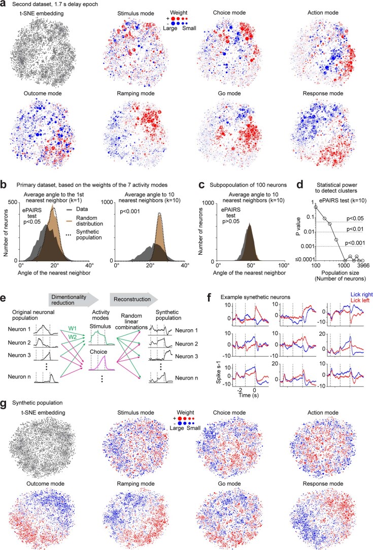
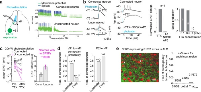
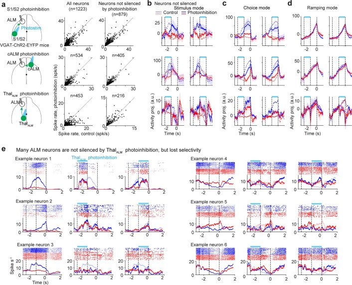
Neurons in frontal cortex exhibit diverse selectivity representing sensory, motor and cognitive variables during decision-making. The neural circuit basis for this complex selectivity remains unclear. We examined activity mediating a tactile decision in mouse anterior lateral motor cortex in relation to the underlying circuits. Contrary to the notion of randomly mixed selectivity, an analysis of 20,000 neurons revealed organized activity coding behavior. Individual neurons exhibited prototypical response profiles that were repeatable across mice. Stimulus, choice and action were coded nonrandomly by distinct neuronal populations that could be delineated by their response profiles. We related distinct selectivity to long-range inputs from somatosensory cortex, contralateral anterior lateral motor cortex and thalamus. Each input connects to all functional populations but with differing strength. Task selectivity was more strongly dependent on thalamic inputs than cortico-cortical inputs. Our results suggest that the thalamus drives subnetworks within frontal cortex coding distinct features of decision-making.

Fig. 1. Diverse yet repeatable response profiles in ALM.

a, Mice reporting the location of a pole by directional licking after a delay epoch. b, Silicon probe recording and example neurons. Left ALM. Top: spike raster. Bottom: PSTH. Blue, ‘lick right’ trials; red, ‘lick left’. Dashed lines, behavioral epochs as in a. c, Analysis of diverse response profiles. Individual neuron PSTHs of ‘lick right’ (blue) and ‘lick red’ trials (red) are concatenated. The population response is reduced to the top 50 principal components and embedded into a two-dimensional t-SNE. Dots, individual neurons. Only neurons showing consistent modulation during the task are included (n = 7,340 neurons, 73 mice). Neurons are divided into 94 clusters. Colors show two clusters. PC, principal component. d, PSTHs of individual neurons in the example clusters in c. e, Rows 1–2: PSTHs (mean ± s.e.m. across neurons) of eight example clusters in the primary dataset. Rows 3–4: PSTHs of matching clusters from a second dataset (n = 8,736 neurons, 29 mice). t-SNE and clustering are performed independently on the second dataset, resulting in 86 clusters. f, Left: response profiles of all clusters from the primary dataset. Each row shows activity of one cluster. Right: response profiles of the second dataset. g, Fraction of neurons falling into each cluster in the primary dataset (thick line). Clusters are ranked based on size. Gray lines, fraction of neurons in four distinct mouse groups (18 mice each; n = 1,628, 2,095, 1,547, 1,984 neurons, respectively). Dots, fraction of neurons in matched clusters from the second dataset. The position of the dots on the x axis is based on the matching cluster from the primary dataset. h, Noise correlation for simultaneously recorded neuron pairs. n = 1,060 pairs from the same cluster (filled symbols); n = 1,598 pairs from different clusters (open symbols) (Methods). Noise correlation is trial-to-trial cofluctuations in the mean-subtracted spike rate. See Extended Data Fig. 1i for noise correlation during specific task epochs. Mean ± s.e.m. across neuron pairs. ***P = 1.82 × 10⁻⁴⁹, two-sided Wilcoxon rank sum test, within-cluster pairs versus across-cluster pairs. ‘Lick right’ and ‘lick left’ trials are combined for the test.

Fig. 2. Task and behavioral information is represented by distinct activity modes.

a, Decoding accuracy for stimulus (trial type instructed by object location), choice (lick direction), outcome (rewarded versus unrewarded), trial epoch (baseline, sample, delay, response), reaction time (fast versus slow trials) and ignore trials. Decoding is performed independently at each time point on population responses generated from different combinations of single neuron trial data (mean ± s.d. across runs, Methods). Only neurons with more than ten error trials of each trial type are included (n = 2,039). b, Left: neural trajectories and selectivity directions in activity space. Error trial trajectories distinguish stimulus versus choice selectivity. Right: correlation of stimulus and choice selective directions across time. Bounding boxes, activity modes are selective directions in specific epochs. Green, stimulus mode. Magenta, choice and action modes. Only neurons with more than five error trials of each trial type are included (n = 3,966). c, ALM population activity along specific activity modes in correct trials. Mean ± s.e.m. (bootstrap, Methods). Blue, ‘lick right’ trials instructed by object location; red, ‘lick left’ trials. Percentage of activity variance captured is shown at top. d, Activity projection in error trials. Mean ± s.e.m. (bootstrap, Methods). Light blue, ‘lick right’ trials instructed by object location, but mice licked left; light red, ‘lick left’ trials in which mice licked right. e, Activity projection in ignore trials. Mean ± s.e.m. (bootstrap, Methods). Activity modes are computed separately from c and d using neurons with more than two ignore trials of each trial type (n = 546). Dashed lines, activity in correct trials. Dark blue, ‘lick right’ trials instructed by object location; dark red, ‘lick left’ trials. f, Activity projection in trials in which mice licked before the go cue. Activity is aligned to the first lick. Mean ± s.e.m. (bootstrap, Methods). Only neurons with more than three early lick trials of each trial type are included (n = 1,994). Also see Extended Data Fig. 3. g, Left: activity projection separately by fast or slow reaction time. Top and bottom 1/3 of trials sorted by reaction time. Correct trials only. The x axis is the same as in panels c and d. Mean ± s.e.m. (bootstrap, Methods). Right: activity projection during the last 200 ms of the delay epoch. Trials with the fastest (top 1/3), intermediate (middle 1/3) and slowest reaction times (bottom 1/3). Mean ± s.e.m. (bootstrap, Methods). Only neurons with more than five error trials and more than two trials of each reaction time condition are included (n = 3,918). *P = 0.002; ***P = 5.06 × 10⁻¹⁴, two-tailed t-test. a.u., arbitrary units; RT, reaction time.

Fig. 3. Activity modes coding stimulus, choice and action are supported by distinct neuronal populations.

a, Activity modes correspond to weighted sums of individual neuron activities. The weights show contribution of individual neurons. b, Neuron weights in the t-SNE. Dots, individual neurons. Dot size shows weight magnitude and colors indicate positive (red) or negative (blue) weights. Only neurons with more than five error trials of each trial type are included (n = 3,966). c, Top: a seven-dimensional vector represents each neuron’s contributions to the activity modes. For neuronal populations with random mixtures of selectivity, coding vectors are uniformly distributed around the origin, which can be quantified by angles between nearest neighbors (ePAIRS test). Bottom: the distribution of angles deviates significantly from random distribution of coding vectors and from a synthetic population coding random mixtures of activity modes, indicating that distinct task selectivity is not randomly mixed within ALM populations. P < 1 × 10⁻⁴, one-sided test (Methods). d, A two-dimensional vector represents each neuron’s contributions to a pair of activity modes. If neurons encode random mixtures of each activity mode, rather than encoding one mode or another, these vectors are uniformly distributed. Neuronal populations coding single activity modes are located around 0° and 90°. Neural coding of stimulus, choice and action exhibits significant peaks at 0° and 90°. In contrast, coding of choice and ramping shares the same neuronal population. Dashed line, synthetic population coding mixtures of activity modes. Stimulus and choice, P = 0.0018; choice and action, P = 4.40 × 10⁻⁶; stimulus and action, P = 2.27 × 10⁻⁹; ramping and choice, P = 0.19, Kolmogorov–Smirnov test, observed distribution versus synthetic population, one-sided test. e, Left: k-means clustering on activity mode weights delineates neurons into six clusters (Methods). Right: clusters shown in the t-SNE. Clusters carrying the most variance for the stimulus, choice and action modes are termed stimulus, choice and action coding (Extended Data Fig. 5a). f, Classification of stimulus, choice and action coding neurons using a nearest-neighbor classifier in the t-SNE (Methods). Mean ± s.e.m. (bootstrap across neurons). Only neurons with more than five error trials of each trial type are included (n = 3,966). g, Distribution of stimulus, choice and action coding neurons across depth. Fraction is relative to all neurons from each functional population (stimulus coding, n = 583 neurons/73 mice; choice coding, n = 694 neurons/73 mice; action coding, n = 491 neurons/73 mice). Mean ± s.e.m. across mice (dots). K-S, Kolmogorov–Smirnov test; W, weight.

Fig. 4. ALM receives long-range inputs from S1/S2, cALM and Thal_ALM which are required for behavior.

a, Retrograde and anterograde tracing from ALM. Left: labeling in ipsilateral S1/S2, cALM and ipsilateral Thal_ALM. Right: magnified images. Red, retrograde labeling (WGA-Alexa594); green, anterograde labeling (GFP); blue, Nissl stain. Retrograde and anterograde tracings were performed in the same brain. This experiment was repeated in five mice with similar results. b, Behavioral performance in the tactile decision task with photoinhibition of left S1/S2 (top), right ALM (middle) or left Thal_ALM (bottom) during different trial epochs. Thick lines, mean; thin lines, individual mice (S1/S2, n = 6; cALM n = 4; Thal_ALM, n = 5). S1/S2, *P = 0.012; cALM, **P = 0.0016; Thal_ALM, *P = 0.015, ***P = 0.0001; P values obtained by nested bootstrap across mice, sessions and trials, one-sided test (Methods). Ctrl, control.

Fig. 5. S1/S2, cALM and Thal_ALM inputs connect to all response profiles in ALM.

a, Measuring long-range input connectivity using ChR2-tagging. b, Top: example neurons with short-latency responses to photostimulation of S1/S2 axons (tagged). Bottom: example ALM neurons unresponsive or suppressed by photostimulation (nontagged). Photostimulus, 1-ms pulses, 30 mW. c, Top: average response of tagged (n = 172) and nontagged neurons (n = 1,487). S1/S2, cALM and Thal_ALM axonal photostimulation data are combined. Bottom: response magnitude and latency of tagged neurons. Box and whisker plot shows median, 25/75th percentiles and most extreme data points not considered as outliers. d, ChR2-assisted circuit mapping. e, Calibration recordings from ALM. Left: example EPSPs. S1/S2 axonal photostimulation. Application of TTX left EPSP intact in a connected neuron (top). TTX abolished EPSP in an unconnected neuron (bottom). Right: mean EPSP before and after TTX for all tested neurons. Photostimulation power, 20 mW. f, EPSP latency of neurons verified to be connected or unconnected using TTX. Mean ± s.d. across neurons (S1/S2, n = 17; cALM, n = 17; Thal_ALM, n = 13). A latency threshold (5 ms) could differentiate connected and unconnected neurons. Dots, individual neurons. Unconnected neurons with no EPSPs are shown on top. g, Left: ALM neurons connected to S1/S2 (top), cALM (middle) and Thal_ALM inputs (bottom) shown in the t-SNE. Colored dots, connected neurons measured from ChR2-tagging (red) and ChR2-assisted circuit mapping (black); gray dots, all neurons in the dataset. Only a subset of the neurons are tested for input connectivity. Right: fraction of connected neurons relative to all tested neurons within each functional population (Fig. 3e). Box and whisker plot shows median, 25/75th percentiles and most extreme data points not considered as outliers (bootstrap, Methods). h, S1/S2, cALM and Thal_ALM inputs differed in strength. Left: connection probability from ChR2-assisted circuit mapping. Numbers on each bar indicate the number of tested neurons. Right: light-induced EPSP in the connected neurons. Mean ± s.e.m. across neurons (dots). S1/S2, n = 43; cALM, n = 53; Thal_ALM, n = 45. Only a subset of the neurons in panel h are tested in behavior, shown in panel g. See Extended Data Fig. 8. VM, ventral-medial nucleus.

Fig. 6. Thalamic inputs drive all response profiles in ALM.

a, Effects of photoinhibiting S1/S2 (top), cALM (middle) and Thal_ALM (bottom) on ALM spike rates. Neurons are tested for significant spike rate change (Methods). Data from sample and delay epoch photoinhibition are combined. ‘Lick left’ and ‘lick right’ trials are pooled. Mean ± s.e.m. across mice (dots). S1/S2 photoinhibition, layer 2/3, n = 55 neurons; layer 5, n = 543; layer 6, n = 383, 12 mice. cALM photoinhibition, layer 2/3, n = 27; layer 5, n = 243; layer 6, n = 174, 10 mice. Thal_ALM photoinhibition, layer 2/3, n = 15; layer 5, n = 193; layer 6, n = 169, 9 mice. b, Effects of photoinhibiting S1/S2 (top), cALM (middle) or Thal_ALM (bottom) on ALM functional populations. Left: excited (red dots) or silenced (blue dots) neurons shown in the t-SNE. Dot size represents the magnitude of spike rate change during photoinhibition relative to control. Gray dots, all neurons in the dataset. Only a subset of the neurons are tested for photoinhibition. Right: fraction of excited and inhibited neurons relative to all tested neurons within each functional population. Only neurons with spike rates greater than 0.5 and tested for more than five error trials of each trial type are included. S1/S2 photoinhibition: n = 59, 63, 32 neurons, 12 mice, for stimulus, choice and action coding populations; cALM photoinhibition, n = 51, 56, 23 neurons, 10 mice; Thal_ALM photoinhibition, n = 44, 47, 18 neurons, 9 mice. Mean ± s.e.m. across mice (dots). Also see Extended Data Fig. 9. L, layer.

Fig. 7. Activity modes coding stimulus and choice require thalamic inputs.

a, Effects of photoinhibiting S1/S2 (top), cALM (middle) and Thal_ALM (bottom) on ALM stimulus mode. Mean ± s.e.m. (bootstrap, Methods). Dotted lines, activity in control trials. Dashed lines delineate behavioral epochs. Both correct and error trials are included in activity projections, grouped by instructed trial type. Blue, ‘lick right’ trials; red, ‘lick left’ trials. b, Same as a but for ALM choice mode. Mean ± s.e.m. (bootstrap, Methods). c, Same as a but for ALM ramping mode. Mean ± s.e.m. (bootstrap, Methods). d, Changes in ALM activity modes during photoinhibition relative to control trials. Activity changes in ‘lick left’ and ‘lick right’ trials are averaged. Data from sample and delay epoch photoinhibition are combined. Only neurons with more than five error trials and at least two photoinhibition trials for each trial type are included (S1/S2, n = 326; cALM, n = 310; Thal_ALM, n = 208). Box and whisker plot shows median, 25/75th percentiles and most extreme data points not considered as outliers. Thal_ALM versus S1/S2, P = 0.039, 0.001, 0.11, <1 × 10⁻⁴, 0.003, 0.025, 0.011 for stimulus, choice, action, outcome, ramping, go, response modes, respectively; Thal_ALM versus cALM, P = 0.065, 0.016, 0.059, 0.003, 0.005, 0.098, 0.019. P values obtained by bootstrap, one-sided test (Methods).

Fig. 8. Action mode and movement initiation require thalamic inputs.

a, Direct photoinhibition of Thal_ALM using GtACR1. Injection of AAV Cre virus in a Cre-dependent GtACR1 reporter mouse. Red, expression of GtACR1 in Thal_ALM. This experiment was repeated in seven mice with similar results. b, Effect of photoinhibiting Thal_ALM on ALM action mode. Dotted lines, activity in control trials. Dashed lines delineate behavioral epochs. Correct, error and ignore trials are combined, grouped by instructed trial type. Blue, ‘lick right’ trials; red, ‘lick left’ trials. Photostimulation power, 1–3 mW. c, Left: lick rate in control and Thal_ALM photoinhibition trials (n = 5 mice). Right: fraction of ignore trials in control and Thal_ALM photoinhibition trials. Thick lines, mean; thin lines, individual mice. ***P < 1 × 10⁻⁴; P value obtained by nested bootstrap across mice, sessions and trials, one-sided test (Methods).

Extended Data Fig. 1. Prototypical response profiles in ALM.

a Example clusters from the primary dataset. Left, dots represent individual neurons in the t-SNE representation. Neurons are divided into 94 clusters. Colors indicate 7 example clusters. Right, PSTHs of individual neurons in the example clusters. b ePAIRS test for distribution of response profiles. Each neuron’s PSTH shape is represented by a 26-dimensional vector that contains the loadings of the top 26 principal components of the population activity. For continuous variation of response profiles (that is no clustering), the vectors are uniformly distributed around the origin, which can be quantified by computing the angle between nearest neighbors (ePAIRS test). The distribution of angles deviates significantly from uniform distribution (P <1 × 10⁻⁴ for k=1, P < 1 × 10⁻⁴ for k=10, one-sided test, Methods), indicating that ALM response profiles exhibit clusters of prototypical response profiles. The result is consistent across different number of nearest neighbors (k) used to calculate average angle. c Cell-cell co-clustering matrix for every pair of neurons in the primary dataset. Only neurons showing consistent modulation during the task are included (n = 7340 neurons, 73 mice). Neurons are sorted based on density peak clustering (left). Co-clustering matrix of the same neuron pairs is shown for Louvain-Jaccard clustering (right). The block structure along the matrix diagonal is preserved in Louvain-Jaccard clustering, indicating that if two neurons belong to the same cluster by density peak clustering, then their co-clustering probability is high for Louvain-Jaccard clustering. d Average PSTHs of the largest and smallest clusters from the primary dataset. Mean ± SEM across neurons. The largest clusters are reproducible in Louvain-Jaccard clustering. The small clusters are not reproduced. e Robustness of the clustering results. Left, number of clusters from density peak clustering as a function of population size. Neurons are subsampled. Mean ± S.D. across populations. Cluster number saturates rapidly after 1000 neurons. Dashed line, the primary dataset consists of 94 clusters after manual merging of some similar clusters (Methods). Right, reproducibility of clusters in Louvain-Jaccard clustering. For each cluster from density peak clustering, we quantified the fraction of its units captured by a matching cluster in Louvain-Jaccard clustering (Methods). Clusters with >0.5 of units captured are considered reproducible. f Clusters from the second dataset are matched to clusters from the primary dataset based on the similarity their PSTHs. The plot shows Pearson’s correlation between clusters from the second dataset with all the clusters from the primary dataset. Clusters are matched based on high correlation coefficient (Methods). This analysis focuses on 48 clusters from the second dataset that are most readily matched to a corresponding cluster in the primary dataset. Gray lines, individual clusters; black line, mean. g Average PSTHs of 8 example clusters. Mean ± SEM across neurons. Rows 1–4 show distinct mouse groups (n = 18 mice per group). Row 5 shows matching clusters from the second dataset. h Response profiles of all clusters from 4 distinct mouse groups. Each row shows average activity of one cluster. i Neuron pairs with similar response profiles exhibit noise correlation. Top, an example neuron pair from the same cluster. Spike raster and PSTHs show simultaneously recorded responses from the neuron pair. In trials where one neuron exhibits high spike rate, the other neuron also exhibits high spike rate. The two neurons are 200 µm apart. Bottom, noise correlation for all neuron pairs. Mean ± SEM across neuron pairs. Same as Fig. 1h but for noise correlation calculated in various epochs. Baseline, = 1.98 × 10⁻¹¹; sample, P = 1.94 × 10⁻³⁰; delay, P = 8.91 × 10⁻³⁵; response, P = 9.92 × 10⁻¹⁵, two-sided Wilcoxon rank sum test (Methods).

Extended Data Fig. 2. Activity modes are highly robust across mice, conditions, and analysis Methods.

a Angles between activity modes. The activity modes are near orthogonal to each other. b Activity and selectivity variance explained by each activity mode. Activity and selectivity variance are computed using trial-averaged activity during specific epochs (Methods), thus they reflect variance across time and neurons. Variance across trials is not reflected. c Activity modes are highly robust across mice, conditions, and decomposition methods. The plots show ALM activity projections on specific activity modes. Solid colors, correct trials; transparent colors, error trials. Blue, ‘lick right’ trials instructed by object location; red, ‘lick left’ trials. Row 1–4, activity modes from 4 distinct mouse groups in the primary dataset. Only neurons with more than 5 error trials of each trial type are included (n = 988, 767, 972, 1200 respectively). Mean ± SEM (bootstrap, Methods). Row 5, activity modes from simultaneously recorded populations (33 sessions, 10–57 neurons per session, average 24 neurons). Mean ± SEM across sessions. Row 6, activity modes from the second dataset (n = 4010 neurons). Mean ± SEM (bootstrap, Methods). Row 7, activity modes from demixed principal component analysis (demixed PCA) on the primary dataset. The top activity modes discovered by demixed PCA correspond to stimulus, choice, action, outcome, ramping, go, and response mode. The percentage of activity variance captured by each activity mode is shown on top. d Additional activity modes obtained from demixed PCA ranked by their activity variance. Together, the 14 activity modes from demixed PCA shown here captured 99.47% of activity variance.

Extended Data Fig. 3. Correlation of activity modes with behavior.

a Activity projections in correct, error, and early lick trials. Activity is aligned to the go cue for correct and error trials. Activity is aligned to the time of the first lick for early lick trials. Only neurons with more than 3 early lick trials of each trial type are included (n = 1994). Mean ± SEM (bootstrap, Methods). b Left, reaction time in correct trials with the fastest (top 1/3), intermediate (middle 1/3), and slowest reaction time (bottom 1/3). Box-whisker plot, box edges, 75 and 25 percentiles, whiskers, extremities of data not considered as outliers, black bars, median. n = 132,907 trials/85 mice. Right, activity projections during the last 200 ms of the delay epoch. Only neurons with more than 5 error trials of each trial type and more than 2 trials of each reaction time condition are included (n = 3918). Choice mode, **P = 0.0014; ***P = 3.22 × 10⁻⁵, two-tailed t-test. Ramping mode, *P = 0.002; ***P = 5.06 × 10⁻¹⁴, two-tailed t-test.

Extended Data Fig. 4. Activity modes are non-randomly mixed across ALM populations.

a Neuron weights in the t-SNE representation. Same as Fig. 3b, but for the second dataset. b Distribution of coding vector angles between nearest neighbors. Same as Fig. 3c, but for different number of nearest neighbors (k) used to calculate average angles (ePAIRS test, one-sided test; P = 0.049 for k=1, P < 1 × 10⁻⁴ for k=10, Methods). Data from the primary dataset. Only neurons with more than 5 error trials of each trial type are included (n = 3966). c Effect of neuronal population size on analysis of mixed selectivity. 100 neurons are randomly selected from the full dataset to generate subpopulations. The histogram shows the distribution of coding vector angles between nearest neighbors in the subpopulation (P = 0.54, ePAIRS test, one-sided test). The distribution is not significantly different from random distribution. Thus a population of 100 neurons appears to exhibit randomly mixed selectivity. d Power analysis showing the P value of ePAIRS test as a function of population size. Subsets of neurons are randomly selected from the full dataset to generate subpopulations. Detecting significant deviations from randomly mixed selectivity using a criterion of P < 0.01 (one-sided test) requires at least 400 neurons. e Generation of a synthetic population in which the coding of activity modes is randomly mixed. Each synthetic neuron’s PSTH is constructed from random combinations of the activity modes and eigenvectors of the original population response. This procedure preserved the activity modes but redistributed them randomly across the synthetic population. f PSTHs of example synthetic neurons. Blue, ‘lick right’ trials; red, ‘lick left’ trials. g Neuron weights in the t-SNE representation. Same as Fig. 3b, but for the synthetic population.

Extended Data Fig. 5. Functional populations.

a Neurons in the primary dataset are divided into 6 functional populations using k-mean clustering on the weights of the 7 activity modes (Methods). Left, different functional populations in the t-SNE representation. Right, fraction of variance carried for each activity mode. For each activity mode, the fraction of variance across all 6 functional populations adds up to 1. Most functional populations carry the majority of variance for single activity modes. Functional populations that carry the most variance for the stimulus, choice, and action modes are termed stimulus, choice, and action coding. Choice coding population also carries most of the variance for the ramping mode. Action coding population also carries most of the variance for the go mode. The response mode is more evenly distributed across different functional populations. Only neurons with more than 5 error trials of each trial type are included (n = 3966). b Same as (a) but for the second dataset. n = 4010 neurons. c Same as (a) but for the synthetic population in which the coding of activity modes is randomly mixed. n = 3966 synthetic neurons. d Distribution of functional populations across depth. Open bars, distribution of specific functional populations; gray bars, distribution of all neurons in the dataset. Silicon probe recordings preferentially sample neurons from the deep layers. The distribution of each functional population does not differ from the distribution expected from sampling (gray). Neurons from the primary dataset. e Left, putative pyramidal neurons (gray dots) and fast-spiking interneurons (red dots) in the t-SNE representation. Interneuron responses are also diverse and span all prototypical response profiles observed in ALM. Right, average PSTHs of pyramidal neurons (top) and interneurons (bottom) in example clusters. Mean ± SEM across neurons. Interneurons exhibit similar PSTHs as the pyramidal neurons, but exhibit less trial-type selectivity.

Extended Data Fig. 6. ChR2-assisted circuit mapping and validation.

a Left, calibration whole-cell recordings measuring vS1→vM1 connectivity using ChR2-assisted circuit mapping. Right, recordings from two example vM1 neurons during photostimulation of vS1 axons. The traces show 15 mins of recordings after TTX application. Green, membrane potential; blue, action potentials. TTX left EPSPs intact in the connected neuron (top, see light-induced EPSPs in the green trace after action potentials were eliminated). TTX abolished EPSPs in the unconnected neuron (bottom). b Pharmacology to verify synaptic connections. Left, photostimulation of vS1 axons elicits short-latency EPSPs in vM1 neurons. Application of TTX left EPSPs intact in a connected neuron (top). TTX abolished EPSPs in an unconnected neuron (bottom). Middle, data from a connected neuron. Application of TTX left EPSPs intact. Application of AMPAR antagonist NBQX and NMDAR antagonist AP5 abolished the remaining EPSPs, confirming that the remaining EPSPs resulted from synaptic depolarization. Thin lines, individual photostimulation repetitions; thick lines, mean. Right, data from all recordings tested with TTX, NBQX and AP5. Neurons tested with TTX, NBQX and AP5, n = 4; neurons tested with various TTX concentrations, n = 19. c Left, mean EPSP before and after TTX for all tested vM1 neurons. Right, EPSP latency of all vM1 neurons verified to be connected or unconnected using TTX. Mean ± SD across neurons (n = 28 neurons). Dots, individual neurons. Photostimulation power, 20 mW. Unconnected neurons with no EPSPs are shown on top. The EPSP latencies in vM1 neurons are overall faster than ALM neurons (Fig. 5f). Nevertheless, connected and unconnected neurons could be differentiated based on latency. d Left, connection probability of vS1 inputs in vM1 superficial (<570 µm) and deep layers (>570 µm). vS1 inputs preferentially excite vM1 superficial layers, consistent with. Right, connection probability of M2 inputs to vM1 inputs. M2 inputs preferentially excite vM1 deep layers, consistent with. e Limited anterograde infection of ALM neurons from virus injections in S1/S2, cALM, and Thal_ALM. Left, an example confocal image showing an ALM section 2 months after virus injection in S1/S2. Red, NeuN; green, ChR2 expression in S1/S2 input axons. Arrows indicate rare ALM neurons with ChR2 expression. Right, fraction of ALM neurons showing ChR2 or ReaChR expression for virus injections in S1/S2, cALM, and Thal_ALM (n = 3 mice each, 2–3 months after virus injection). The lack of ChR2 or ReaChR expression indicates that the light-induced EPSPs are due to ChR2 or ReaChR expressing long-range input axons. Scale bar, 10 µm.

Extended Data Fig. 7. Connectivity and intrinsic properties of ALM neurons.

a Connected (solid dots) and unconnected neurons (open dots) measured from ChR2-assist circuit mapping shown in the t-SNE representation. b Same as (a) but for connected neurons measured from ChR2-tagging. c Firing patterns of ALM neurons do not predict long-range input connectivity. Left, example firing patterns in response to current injections during whole-cell recording. Neurons are classified into regular spiking, bursting, and high threshold types (Methods). Middle, regular spiking (black), bursting (brown), and high threshold neurons (red) shown in the t-SNE representation. Right, classification flow chart of connected neurons to regular spiking, bursting, and high threshold types. d EPSP dynamics of ALM neurons do not predict long-range input connectivity. Left, example light-induced EPSPs. Neurons are classified into facilitating, depressing, and indirect/inhibitory types based on EPSP dynamics. Middle, neurons with facilitating (black), depressing (purple), and indirect/inhibitory responses (green) in the t-SNE representation. Right, classification flow chart of connected neurons to facilitating, depressing, and indirect/inhibitory responses. e Membrane time constant of ALM neurons does not predict long-range input connectivity. Left, example neurons with short and long time constant. Tau is measured as the time when EPSP decays to 67% of its peak amplitude after a 1-ms depolarizing or hyperpolarizing current injection. Middle, neurons with different time constant in the t-SNE representation. Right, classification flow chart of connected neurons to different time constant.

Extended Data Fig. 8. Connectivity patterns of S1/S2, cALM, and Thal_ALM inputs.

a Connection probability across depth measured from whole-cell recording and ChR2-assisted circuit mapping. Left, data from untrained mice, in which connections are verified with TTX pharmacology. Right, data from mice trained in the tactile decision task, in which connections are inferred by EPSP latency. Only a subset of the neurons was held long enough to be tested further in the tactile decision task (Fig. 5g and S7). Numbers on each bar indicate the number of tested neurons. b Connection strength measured from whole-cell recordings. Mean ± SEM across neurons (each dot represents one neuron). Untrained mice, S1/S2, n = 16 neurons; cALM, n = 28 neurons; VM, n = 28 neurons. Trained mice, S1/S2, n = 27 neurons; cALM, n = 25 neurons; VM, n = 17 neurons. A range of photostimulation power (1, 5, 10, 20 mW) and pulse conditions (1, 3, 5, 10 pulses; 2-ms pulses at 5-ms interval) were tested. Photostimulation of Thal_ALM axons elicits the strongest EPSP (between S1/S2 or cALM and VM, P = 1.86 × 10⁻⁸, untrained group; P = 8.82 × 10⁻¹⁴, trained group, two-way ANOVA, powers and inputs).

Extended Data Fig. 9. Direct Thal_ALM photoinhibition using GtACR1.

a Direct photoinhibition of Thal_ALM using GtACR1. Top, injection of AAV Cre virus in Thal_ALM of a Cre-dependent GtACR1 reporter mouse. Green, expression of eGFP-Cre. Red, GtACR1 expression. Autofluorescence around optical fiber track is visible in green. After mice were tested in Thal_ALM photoinhibition, optical fiber implants were removed. Optrode recordings were made in Thal_ALM (left) and posterior thalamus (right) to characterize the spatial specificity of Thal_ALM photoinhibition. For posterior thalamus, recording tracks were labeled with DiI (arrow in the right image). Recordings were performed in awake non-behaving mice (n = 2). Bottom, example voltage traces and average activity of neurons in Thal_ALM and posterior thalamus. Photostimulation power, 1 mW. b Effect of direct Thal_ALM photoinhibition on cortical activity. Left column, silicon probe recordings in ALM (coordinates from bregma: anterior 2.5 mm, lateral 1.5 mm; n = 113, 2 mice) and S1 (posterior 1.0 mm, lateral 3.1 mm; n = 165, 2 mice). The image shows expression of eGFP-Cre (green) and GtACR1 (red) in Thal_ALM. Recording tracks were labeled with DiI (arrow). Middle column, Thal_ALM photoinhibition reduced the spike rate in ALM, but not in S1. Average spike rates aligned to photostimulation. Black, control; cyan, photostimulation. Mean ± SEM across neurons. Right column: neurons with significant spike rate change, defined as P < 0.01 using two-tailed t-test between photoinhibition and control trials. Layer 2/3, 110–378 µm (ALM, n = 5 neurons; S1, n = 8); layer 5, 378–772 µm (ALM, n = 45; S1, n = 57); layer 6, below 772 µm (ALM, n = 63; S1, n = 100; Methods). Recordings were performed in awake non-behaving mice. Only neurons with spike rate above 1 Hz are included in the analysis. Mean ± SEM (bootstrap across neurons). Data from 2 mice, the fractions for individual mice are shown as dots. c Effect of direct Thal_ALM photoinhibition on ALM functional populations. Excited (red dots) or silenced (blue dots) neurons shown in the t-SNE representation. Gray dots, all neurons in the dataset (Fig. 1a). Only a subset of the neurons in the dataset are tested for photoinhibition. Photoinhibition is during the sample, delay, or response epoch. Action coding neurons have low spike rates during the sample and delay epoch. Thus photoinhibition during the sample and delay epoch induced limited silencing in this population (Fig. 6b). Here, response epoch photoinhibition strongly silenced action coding neurons. d Distribution of excited and inhibited neurons across functional populations. Fraction is relative to the total number of tested neurons within each functional population. Fraction for stimulus and choice coding populations are from sample and delay epoch photoinhibition. Fraction for action coding population is from response epoch photoinhibition. Mean ± SEM (bootstrap across neurons). Data from 2 mice, the fractions for individual mice are shown as dots. When functional populations are tested during the epoch in which they are active, the fraction of silenced neurons is similar. Stimulus vs. choice coding, P = 0.71; choice vs. action coding, P = 0.36; stimulus vs. action coding, P = 0.48, two-sided chi-square test. e Effect of direct Thal_ALM photoinhibition on ALM activity modes. Mean ± SEM (bootstrap, Methods). Dotted lines show activity projections of control trials. The effects are similar to Fig. 7.

Extended Data Fig. 10. Effects of S1/S2, cALM, and Thal_ALM photoinhibition on ALM activity.

a Spike rates during photoinhibition (1.3 s) versus control conditions. Filled circles, ALM neurons that are significantly modulated by photoinhibition (defined as P < 0.01 using a two-tailed t-test between photoinhibition and control trials). Left column, all neurons. Right column, neurons that retained >50% of the control condition spike rate during photoinhibition. b Effects of photoinhibition on ALM stimulus mode. Activity modes are computed using only neurons that retained >50% of control condition spike rate during photoinhibition. Mean ± SEM (bootstrap, Methods). Dotted lines show activity projections of control trials. Dashed lines delineate behavioral epochs. The effects are similar to Fig. 7. c Same as (b) but for ALM choice mode. Mean ± SEM (bootstrap, Methods). d Same as (b) but for ALM ramping mode. Mean ± SEM (bootstrap, Methods). e Example ALM neurons during Thal_ALM photoinhibition. Spike raster and PSTH. Left, control trials; middle, sample epoch photoinhibition; right, delay epoch photoinhibition. Cyan bars, photostimulation period. Neurons are not silenced by Thal_ALM photoinhibition, but lost selectivity.

References

1. Machens CK, Romo R, Brody CD. Functional, but not anatomical, separation of ‘what’ and ‘when’ in prefrontal cortex. J. Neurosci. 2010;30:350–360. doi: 10.1523/JNEUROSCI.3276-09.2010. - DOI - PMC - PubMed
1. Chandrasekaran C, Peixoto D, Newsome WT, Shenoy KV. Laminar differences in decision-related neural activity in dorsal premotor cortex. Nat. Commun. 2017;8:614. doi: 10.1038/s41467-017-00715-0. - DOI - PMC - PubMed
1. Brody CD, Hernandez A, Zainos A, Romo R. Timing and neural encoding of somatosensory parametric working memory in macaque prefrontal cortex. Cereb. Cortex. 2003;13:1196–1207. doi: 10.1093/cercor/bhg100. - DOI - PubMed
1. Machens CK, Romo R, Brody CD. Flexible control of mutual inhibition: a neural model of two-interval discrimination. Science. 2005;307:1121–1124. doi: 10.1126/science.1104171. - DOI - PubMed
1. Churchland MM, et al. Neural population dynamics during reaching. Nature. 2012;487:51–56. doi: 10.1038/nature11129. - DOI - PMC - PubMed
Publication types