Awake perception is associated with dedicated neuronal assemblies in the cerebral cortex

Abstract

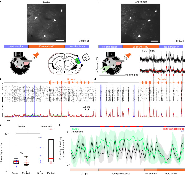
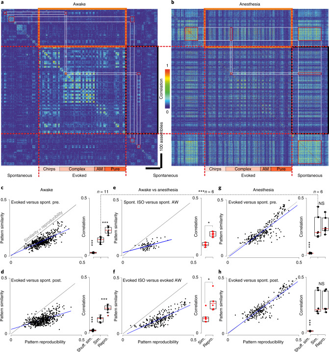
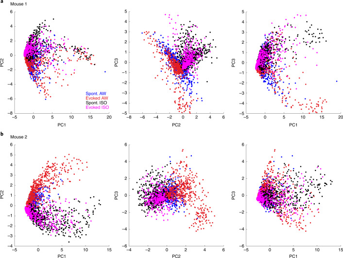
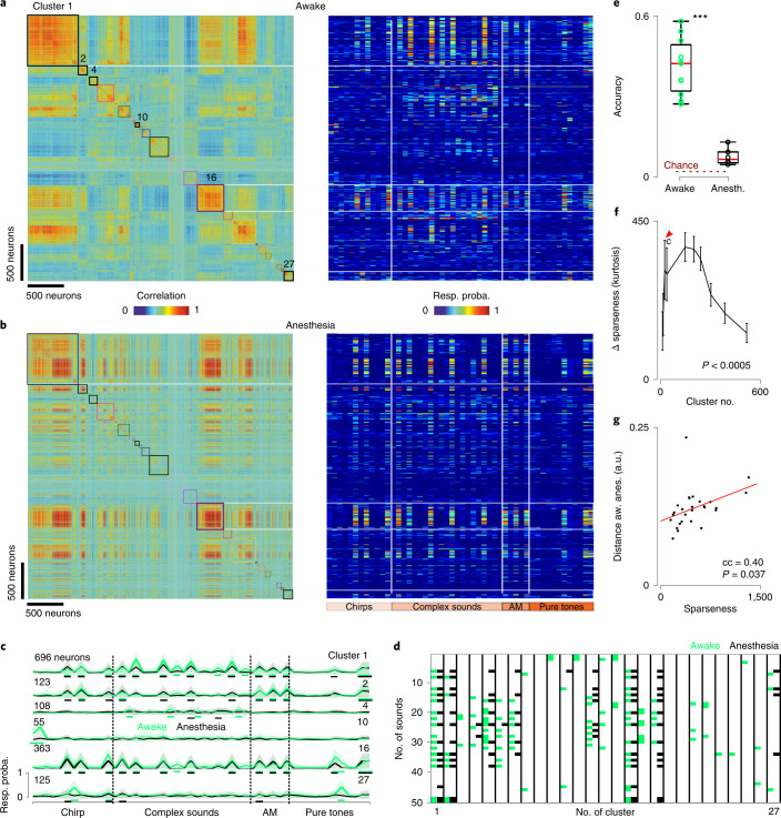
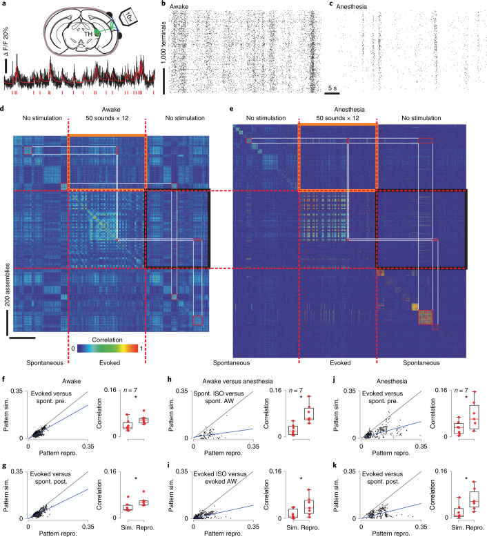
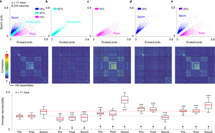
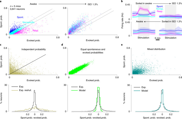
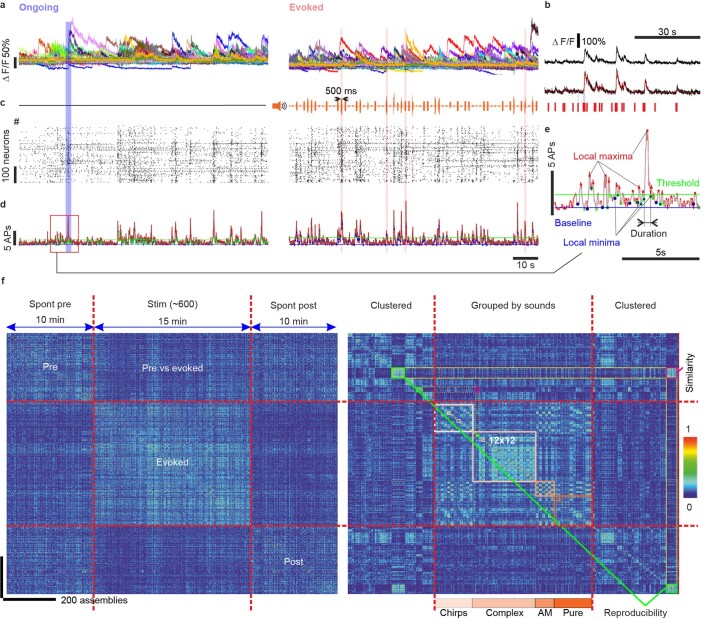
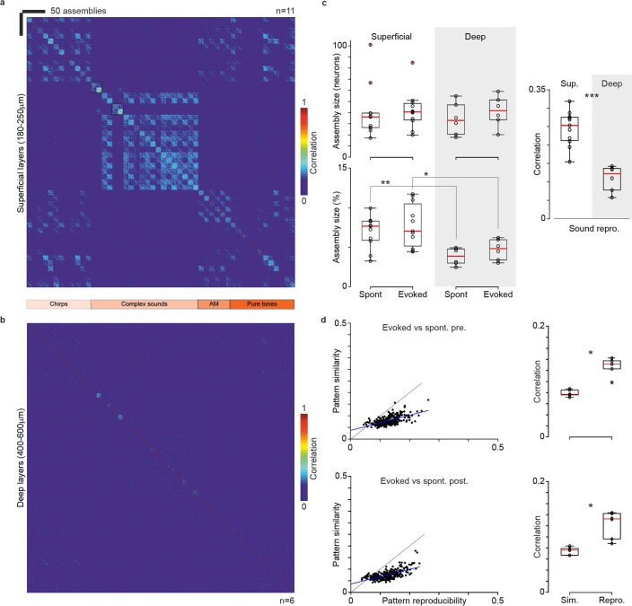
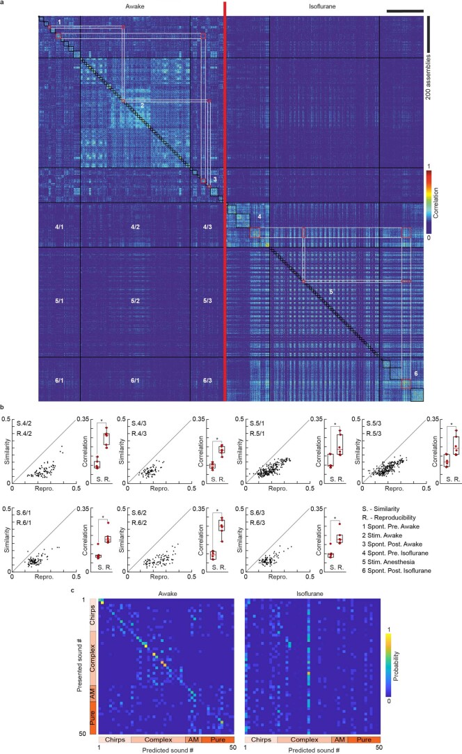
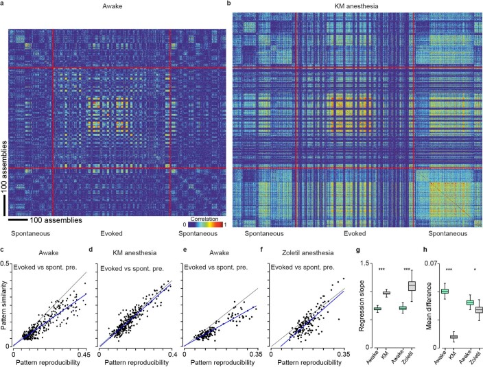
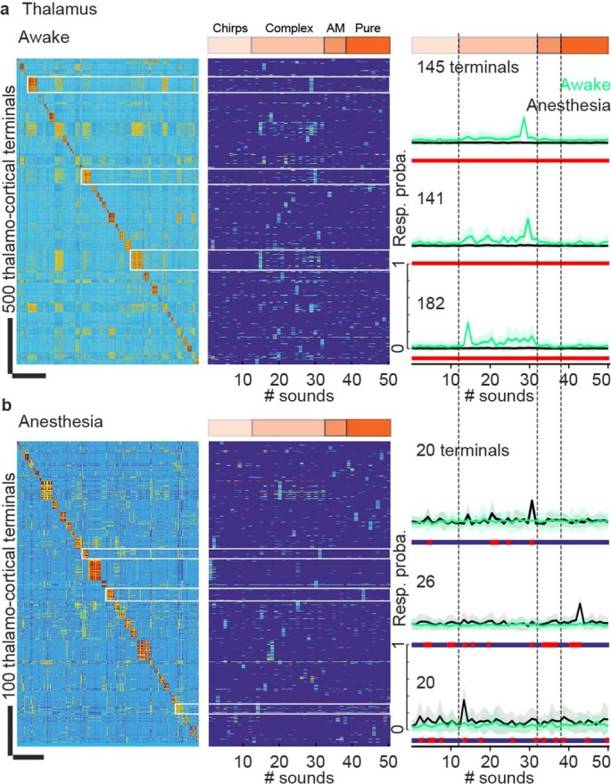
Neural activity in the sensory cortex combines stimulus responses and ongoing activity, but it remains unclear whether these reflect the same underlying dynamics or separate processes. In the present study, we show in mice that, during wakefulness, the neuronal assemblies evoked by sounds in the auditory cortex and thalamus are specific to the stimulus and distinct from the assemblies observed in ongoing activity. By contrast, under three different anesthetics, evoked assemblies are indistinguishable from ongoing assemblies in the cortex. However, they remain distinct in the thalamus. A strong remapping of sensory responses accompanies this dynamic state change produced by anesthesia. Together, these results show that the awake cortex engages dedicated neuronal assemblies in response to sensory inputs, which we suggest is a network correlate of sensory perception.

Fig. 1. Synchronous population events in the auditory cortex in wakefulness and anesthesia.

a, Two-photon Ca²⁺ imaging at a 30-Hz sampling rate of up to 1,200 layer 2/3 neurons expressing GCaMP6s in the awake head-fixed mouse. Upper: imaging field of view with labeled neurons in the awake state showing the s.d. of fluorescence pixels over a 15-min sound stimulation session flanked by two 10-min-long stimulation-free periods. Scale bar, 100 μm. b, The same recording protocol and field of view as in a, but under light isoflurane anesthesia (1.3%). Most neurons are visible in both conditions, demonstrating full stability of the field of view. Weaker or absent labeling in anesthesia reflects neurons that have decreased their activity. Arrows indicate sample neurons. Scale bar, 100 μm. Bottom right: spike time estimates (red) were extracted from calcium fluorescence traces (black) using the MLSpike algorithm. c, Population raster plots and population firing rate (30-ms bins) during no stimulation (left) and stimulation (right) periods. Vertical transparent bars highlight spontaneous (blue) and evoked (pink) population events detected as described in Extended Data Fig. 1d. d, Same as in c but for anesthesia. e, The size of ongoing population events slightly increases under anesthesia (P = 0.036, n = 11 for awake and n = 6 for anesthesia, P = 0.18 for evoked events' Wilcoxon’s rank-sum test). In the box-and-whisker plots, the red mark indicates the median and the bottom and top edges of the box indicate the 25th and 75th percentiles, respectively. The whiskers extend to the extreme data points. f, Probability of sounds evoking population events in the awake state (green trace) and under anesthesia (black trace). The shaded areas indicate the s.d. around the mean. Most of the complex sounds significantly decrease their ability to drive population events (P < 0.05) when passing from wakefulness to anesthesia (Wilcoxon’s rank-sum test for e and f). AM, amplitude modulated; Spont., spontaneous; *P < 0.05; NS, not significant. All tests are two sided. Source data

Fig. 2. Ongoing assemblies and sound-evoked responses differ in the awake state but overlap under anesthesia.

a, For an example recording session, Pearson’s correlation matrix between spontaneous assemblies sorted by hierarchical clustering and single trial sound response patterns (whether or not a population event was detected), sorted sound by sound (12 trials per sound, sound order indicated below). Clustering is done independently in pre- and poststimulation periods. Lower correlation inside black and orange frames (similarity) compared with correlations along the diagonal (reproducibility) indicate that spontaneous and evoked patterns are different. b, Correlation matrix under anesthesia for the same neuronal population as in a. Similar correlation in black and orange frames (similarity) and in the squares along the diagonal (reproducibility) indicates that spontaneous and evoked assemblies are highly similar. c–h, Relationship between reproducibility (abscissa) and similarity (ordinate) of sound-evoked and spontaneous patterns for all sounds and sessions. Statistics across sessions are given on the right-hand-side boxplots. Spontaneous and evoked patterns can be considered dissimilar if their reproducibility is significantly larger than their similarity (gray shows the line for the equality and dark blue the data trend). A significant difference between spontaneous and evoked patterns is seen in awake mice (P = 0.001, Shuffl. Sim. P = 0.0002 (c); P = 0.001, Shuffl. Sim. P = 0.0002 (d); Wilcoxon’s signed-rank test, n = 11 mice), but not under anesthesia (P = 0.44, Shuffl. Sim. P = 0.0002 (g); P = 0.56, Shuffl. Sim. P = 0.0002 (h); Wilcoxon’s signed-rank test, n = 6 mice) where the similarity increased significantly (dashed line, c versus g, P = 0.0003, Wilcoxon’s rank-sum test). Evoked and spontaneous population activity patterns under anesthesia are different from patterns in the awake state (e–f, P = 0.03, P = 0.03; paired Wilcoxon’s sgned-rank test, n = 6 mice). AM, Amplitude-modulated sounds; NS, not significant; Pure, Pure tones; spont., spontaneous; Repro., reproducibility; Shuffl. sim., similarity for shuffled data; Sim., simulated. ^*P < 0.05, ^***P < 0.001. For all box-and-whisker plots, the red mark indicates the median, and the bottom and top edges of the box indicate the 25th and 75th percentiles, respectively. The whiskers extend to the extreme data points. All tests are two sided. ISO, isoflurane; AW, awake; pre., pre-stimulation. Source data

Fig. 3. Assemblies of the awake and anesthetized states span different regions of the population state space.

a, Plot of the localization of ongoing and evoked assemblies in the state in the 3D space defined by the first three PCs of the dataset including all ongoing and evoked assemblies, for one representative recording sample. Anesthesia is with isoflurane. Three 2D projections are shown, from left to right: planes defined by 1st and 2nd PCs, by 2nd and 3rd PCs and by 1st and 3rd PCs. b, Same as a for another sample recording in a different animal. Anesthesia is with isoflurane. Color code: magenta = evoked isoflurane (Evoked ISO), red = evoked awake (Evoked AW), black = spontaneous isoflurane (Spont. ISO), blue = spontaneous awake (Spont. AW).

Fig. 4. Modification of sound tuning between wakefulness and anesthesia.

a, Left: matrix of response profile correlation for 3,641 neurons in six awake mice. The neurons are clustered according to the similarity of their responses (metric: Pearson’s correlation coefficient between response probability profiles for the 50 sounds). Right: response probability (Resp. proba.) profiles for all recorded neurons organized with the clustering presented to the left. b, Same as a under anesthesia. c, Mean response profiles in the awake state (green) and under anesthesia (black) for the six sample clusters labeled in a. Green and black rectangles represent significant responses; error bands represent the s.d. around the mean. d, Colored rectangles denote sounds producing a significant response in neurons of 27 clusters presented in a. A multicomparison one-way ANOVA between the actual responses and a shuffled surrogate of the responses was used for the significance evaluation. e, Average sound prediction accuracy for the 50 sounds in the awake versus the anesthetized (Anesth.) state (n = 11 and 6, P = 0.0002, Wilcoxon’s rank-sum test, ^***P < 0.001). Box-and-whisker plots show the red mark denoting the median, and the bottom and top edges of the box indicating the 25th and 75th percentiles, respectively. The whiskers extend to the extreme data points. f, Difference of sparseness of cluster responses to sounds (that is, kurtosis of response distribution) between awake and anesthetized states, as a function of the granularity number of the clustering algorithm. Positive values indicate higher sparseness in the awake state. All measures are significantly larger than zero (Wilcoxon’s signed-rank test; all P values are <0.0005; n is the number of clusters given on the x axis, mean values ± s.e.m.). g, Difference between sound responses in the awake state and under anesthesia (Distance aw. anes.) as a function of response sparseness for 27 clusters selected in a (P = 0.037, bootstrap test, no multiple comparison adjustment). a.u., arbitrary units; cc, correlation coefficient. All tests are two sided. Source data

Fig. 5. Ongoing and evoked population activity patterns in auditory thalamus differ in both awake and anesthetized states.

a, Schematic of the procedure for two-photon Ca²⁺ imaging of thalamocortical terminals expressing GCaMP6s in layer 1 of the auditory cortex. Below: calcium trace (black) with spike time estimates (red) for a sample terminal. b, Population raster plot in the awake state (each line represents the spontaneous spiking pattern of a thalamocortical terminal). c, Same as b under light isoflurane anesthesia (1.3%). d, For an example recording session, Pearson’s correlation matrix between spontaneous assemblies of thalamocortical terminals sorted by hierarchical clustering and single trial sound response patterns (whether or not a population event was detected), sorted sound by sound (12 trials per sound). e, Same as d under anesthesia. Lower correlation inside black and orange frames (similarity) compared with correlations along the diagonal (reproducibility) indicates that spontaneous and evoked patterns are different. f–k, Relationship between reproducibility (abscissa) and similarity (ordinate) of sound-evoked and spontaneous patterns for all sounds and sessions. Statistics across sessions are given on the histograms on the right-hand side (f–k: P = 0.016, paired Wilcoxon’s sgned-rank test, n = 7 mice). Spontaneous and evoked patterns are dissimilar in both awake (f and g) and anesthetized (j and k) states (gray, line of equality; dark blue, data trend) and neither of them kept similitude passing from one state to another (h–j). AW, awake; ISO, isoflurane anesthesia; post., poststimulation; pre., before stimulation; repro., reproducibility; Sim., similarity; spont., spontaneous; TH, thalamus. ^*P < 0.05. For all box-and-whisker plots, the red mark indicates the median, and the bottom and top edges of the box indicate the 25th and 75th percentiles, respectively. The whiskers extend to the extreme data points. All tests are two sided. Source data

Fig. 6. Specificity of evoked patterns relies on a subset of neurons in the awake state.

a, Top: plot of the probability of responding to any sound versus the probability of being recruited in an ongoing event for 6,310 neurons in 11 mice. The color code indicates whether the neuron prefers ongoing (blue) or evoked (magenta) events or nonspecifically participates in both types of events (cyan, boundaries: ±1 m.a.d. of the probability difference). Middle: for a sample session, Pearson’s correlation matrix was computed with all available neurons. Bottom: average sound and spontaneous event cluster reproducibility. b, Same as a but correlation matrix and reproducibility (mean correlation across assemblies of the same spontaneous cluster or of the same sound) are calculated with nonspecific neurons only (67%). c, Same as a but for sound responsive neurons only (15%). d, Same as a but only for neurons preferring ongoing events (18%). e, Same as a but for all except nonspecific neurons (33%). Post, poststimulation; Pre, before stimulation; prob., probability; Resp, responsive; Spont, spontaneous. ^*P < 0.05, ^**P < 0.01, ^***P < 0.001 respectively. For box-and-whisker plots, the red mark indicates the median, and the bottom and top edges of the box indicate the 25th and 75th percentiles, respectively. The whiskers indicate the most extreme non-outlier data points. Red crosses are outliers. b–e: P = 0.002/0.001/0.001; P = 0.001/0.02/0.001, P = 0.001/0.001/0.001, P = 0.001/0.001/0.001; paired Wilcoxon’s signed-rank test (n = 11 mice). All tests are two sided. Source data

Fig. 7. Specificity of cortical neurons for evoked or ongoing activity is redistributed in anesthesia.

a, Plot of the probability of being recruited in an ongoing event (spont. prob.) plotted against the probability of responding to any sound (evoked prob.) for 3,641 neurons in 5 mice in the awake state (left) and under anesthesia (right). The color code is defined as in the left panel. Under anesthesia, the three color-coded populations converge to a single group with strongly correlated probability of activation in spontaneous and evoked events. b, Top: time course of the mean firing rate profiles in the awake state (left) and under anesthesia (right) for each of the three groups of neurons defined in a for the awake state. Bottom: same as above but when the responsive, spontaneous and nonspecific groups are defined in anesthesia. Error bands indicate the s.d. around the mean. c, Top: same as a but probabilities reshuffled along each axis to show the expected probability distribution for independent participations in ongoing and evoked events. Bottom: corresponding distribution of probabilities difference (ongoing − evoked, 6,310 neurons, in 11 mice). Experimental is black and reshuffled dark khaki. d, Probability distributions for 6,310 surrogate neurons with equal participation probabilities in ongoing and evoked events. e, Probability distributions for 6,310 surrogate neurons with probabilities of participating in spontaneous and evoked activity correlated but not equal (that is, the difference between spontaneous and evoked probabilities is drawn from a continuous Gaussian distribution). Exp., experimental; ISO, isoflurane anesthesia; Nonsp., nonspecific; reshuf., reshuffled; Resp., responsive; Spont., spontaneous.

Extended Data Fig. 1. Identification and clustering of spontaneous and evoked assemblies.

a, Examples of raw calcium fluorescence traces without stimulation (left) and during sound stimulation (right). b, Spikes time estimates (red) were extracted from calcium fluorescence traces (top trace: example raw signal) using the MLSpike algorithm (bottom trace: the raw fluorescent trace adjusted to the baseline fluorescence fluctuations). c, Population raster plots during no stimulation (left) and stimulation (right) periods. Every dot represents a spike estimated as in b. d, Population firing rate (30 ms bins) during no stimulation (left) and stimulation (right) periods. Vertical transparent bars highlight spontaneous (blue) and evoked (pink) population events detected as described in e (inset). e, Identification of spontaneous population events from population firing rate (red trace). Stochastic threshold (green), based on population spiking activity and added to the baseline (blue), to identify the local maxima above the threshold (red dots) in the smoothed population firing rate trace (gray). Local minima (blue and green dots) adjacent to the above threshold local maxima define the beginning and the end of the population event, respectively. All neurons spiking at least once within this interval are included into the population event, defining spontaneous or evoked neural assemblies. f, Left panel: For an example recording session, Pearson’s correlation matrix between spontaneous assemblies (pre- and post-stimulation) and the assemblies evoked by a single trial sound response (50 sounds presented 12 times each) in the order of their appearance during 35-minute recording in awake mouse. Diagonal quadrants show the auto-correlation between the same types of assemblies, lateral quadrants – cross-correlation between different types of assemblies. Right panel: for the same data as in the left panel, similarity matrix in which spontaneous assemblies are sorted by hierarchical clustering and evoked responses (whether or not a population event was detected) are sorted sound-by-sound (12 trials/sound). The mean correlation among the assemblies in a cluster or among the assemblies corresponding to single trial sound responses define the reproducibility of a spontaneous or evoked pattern (green inset). The mean cross-correlation between two groups of patterns defines their similarity (pink inset). Color scale for pattern correlation values (red for 1, dark blue for 0). (AM, amplitude modulated sounds; Pure, Pure tones; Spont, spontaneous; Stim, Stimulation).

Extended Data Fig. 2. Dissimilarity of evoked and ongoing assemblies is robust to clustering methods and parameters.

a, Dendrogram plot of the hierarchical binary cluster trees for spontaneous assemblies before and after stimulation in a sample recording session. The horizontal lines indicate the 4 cophenetic distance thresholds tested in the following panels (0.9, 1, 1.2, 1.5). b-e, Correlation matrix for a sample recording in the awake state. The spontaneous assemblies are sorted by hierarchical clustering with thresholds 1, 2, 3, and 4 (in b, c, d, and e respectively) as defined in a. Red squares in the lateral quadrants indicate the maximum similarity pairs. Red squares in the diagonal quadrants indicate clusters and groups. f, Scatter plot and statistics of similarity vs reproducibility (top: evoked/spont. pre.; bottom: evoked/spont.post.) for each threshold value for the example shown in b-e. Reproducibility of spontaneous and evoked assemblies is significantly higher than the similarity of evoked vs spontaneous assemblies independently of the threshold (all p-values equal to 10⁻⁹, n = 50 pairs of clusters, Paired Wilcoxon Signed Rank Test). g, Same as in f, but for the anesthetized state under isoflurane in the same sample population (all p-values were above 0.05, n = 50 pairs of clusters, Paired Wilcoxon Signed Rank Test:thresholds: 0.6 (p = 0.66, 0.50), 0.8 (p = 0.43, 0.94), 1 (p = 0.80, 0.94) and 1.2 (p = 0.16, 0.09)). h, Sample matrix where evoked assemblies were clustered in the same way as spontaneous ones (instead of grouping by sound). i, Relation between reproducibility (abscissa) and similarity (ordinate) of sound-evoked and spontaneous pre-stimulation assemblies for all sounds and sessions. Statistics across sessions are given in the right-hand-side histograms (p = 0.03, n = 6 mice). j, Same as in i for evoked versus spontaneous assemblies detected post-stimulation (p = 0.03, n = 6 mice). Paired Wilcoxon Signed Rank Test for i and j. (Corr., Correlation; Repro., Reproducibility; Sim., Similarity; spont, spontaneous; *, *** indicate p < 0.05, p < 0.001 respectively). For all box-and-whiskers plots, the red mark indicates the median, and the bottom and top edges of the box indicate the 25th and 75th percentiles, respectively. The whiskers extend to the most extreme data points not considered outliers, and the outliers are plotted individually using crosses. All tests are two-sided.

Extended Data Fig. 3. Dissimilarity of evoked and ongoing assemblies is seen also in deep cortical layers.

a, Pearsons’s correlation matrix averaged across 11 mice for the assemblies evoked by sounds in the upper layers of auditory cortex (180–250 um below cortical surface). b, The same as in a, in deep layers (450–600 um below the cortical surface) averaged across 6 mice. c, Top left: average size (number of neurons) of neuronal assemblies in superficial (11 mice) and deep layers (6 mice). Bottom left: average size of neuronal assemblies in % of all neurons in the FOV in superficial and deep layers (p = 0.005, p = 0.02, Wilcoxon rank sum test). Right: sound evoked responses reproducibility in superficial layers is higher than in the infragranular layers (p = 0.0002, Wilcoxon rank sum test). For all tests in c, n = 11 mice for superficial, and n = 6 mice for deep. d, Dissimilarity of sound-evoked and spontaneous patterns for all sounds and sessions in deep layers. Statistics across sessions are given on the right-hand-side histograms (p = 0.03, p = 0.03, Paired Wilcoxon Signed Rank Test, n = 6 mice). (Repro., Reproducibility; Sim., Similarity; Spont, spontaneous; Sup., Superficial; *,**,*** indicate p < 0.05, p < 0.01, p < 0.001 respectively). For all box-and-whiskers plots, the red mark indicates the median, and the bottom and top edges of the box indicate the 25th and 75th percentiles, respectively. The whiskers extend to the most extreme data points. All tests are two-sided.

Extended Data Fig. 4. Ongoing assemblies during stimulation are also dissimilar to evoked responses.

a, For an example recording session, Pearson’s correlation matrix between spontaneous assemblies sorted by hierarchical clustering and single trial sound response patterns. Spontaneous assemblies detected during stimulation sessions in between evoked responses are clustered in the small white rectangle. Their similarity with evoked and spontaneous pre-stimulation assemblies (big white rectangle) are within orange and red rectangles, respectively. b, Dissimilarity of sound-evoked and spontaneous patterns (SpontStim) detected during stimulation (reproducibility on abscissa and similarity on ordinate). Statistics across sessions are given on the right-hand-side histograms (p = 0.001). c, Similarity of ongoing assemblies observed during the pre-stimulation and stimulation epochs. (p = 0.41, Paired Wilcoxon Signed Rank Test, n = 11 mice in b and c). (NS, not significant; Repro., Reproducibility; Sim., Similarity; Spont, spontaneous; *** indicates p < 0.001). For all box-and-whiskers plots, the red mark indicates the median, and the bottom and top edges of the box indicate the 25th and 75th percentiles, respectively. The whiskers extend to the most extreme data points. All tests are two-sided.

Extended Data Fig. 5. Transition from awake to anesthesia changes both sound-evoked and spontaneous patterns.

a, Correlation matrices for ongoing and evoked assemblies across wakefulness and anesthesia. The numbering of the quadrant describes the different recording conditions. (1) Ongoing assemblies in the awake state, sorted by hierarchical clustering (black rectangles). (2) Single trial sound responses in the awake state, grouped sound-by-sound (black rectangles). (3) Post-stimulation ongoing assemblies in the awake state. (4) Ongoing assemblies under anesthesia, before stimulation. (5) Single trial sound responses under anesthesia (whether or not a population event was detected). (6) Ongoing assemblies under anesthesia, after stimulation. Red rectangles in the top right quadrant outline the similarity between the assemblies detected in the awake and anesthetized states. Numbering in the bottom left quadrant indicates pairwise comparisons (for example 4/1 Spont. Pre. Anesthetized vs Spont. Pre. Awake). b, Plot of awake versus anesthetized assembly similarity against assembly reproducibility. Statistics across sessions are given on the right-hand-side histograms (p = 0.03, Paired Wilcoxon Signed Rank Test, n = 6 mice). c, Confusion matrix (that is probability) of the classifier used in Fig. 4e averaged across the 5 mice in which the same populations were imaged in the awake and isoflurane anesthetized state. (AM, amplitude modulated sounds; Repro., Reproducibility; Pure, Pure tones; * indicates p < 0.05). For all box-and-whiskers plots, the red mark indicates the median, and the bottom and top edges of the box indicate the 25th and 75th percentiles, respectively. The whiskers extend to the most extreme data points not considered outliers, and the outliers are plotted individually using red crosses. All tests are two-sided.

Extended Data Fig. 6. Ongoing assemblies and sound-evoked responses overlap under ketamine-medetomidine and zolazepam-tiletamine anesthesia.

a, For an example recording session, Pearson’s correlation matrix between spontaneous assemblies sorted by hierarchical clustering and single trial sound response patterns (whether or not a population event was detected), sorted sound by sound (12 trials/sound). Clustering is done independently in pre- and post-stimulation periods. Lower correlation inside black and orange frames (similarity) compared to correlations along the diagonal (reproducibility) indicate that spontaneous and evoked patterns are different. b, Correlation matrix under ketamine (50 mg/kg) medetomidine (1 mg/kg) anesthesia (KM) for the same neuronal population as in a. Similar correlation in black and orange frames (similarity) and in the squares along the diagonal (reproducibility) indicate that spontaneous and evoked assemblies are highly similar. c, Relation between reproducibility (abscissa) and similarity (ordinate) of sound-evoked and spontaneous patterns for the 50 sounds and 6 sessions recorded in 3 mice. The unity line in black. Regression line in blue. d, Same as in c, but under KM anesthesia. e-f, Same as in c, d, but for 3 experiments in 3 different mice for Zoletil® (70 mg/kg) anesthesia. g, Slope of the regression lines in c-f. Box plot indicates the 5% confidence interval obtained by bootstrapping 1000 times across data points. For both anesthetics, the bootstrap p-value was <0.001. h, Mean difference between reproducibility and similarity in c-f. The bootstrap p-value was <0.001 for KM and 0.02 for Zoletil. In boxplots of g-h, the central mark indicates the median, and the bottom and top edges of the box indicate the 25th and 75th percentiles, respectively. Distributions were obtained by bootstrapping across data points. The whiskers extend to the most extreme data points. Bootstrapping (1000 random resampling with replacement) was also used to assess the significance of the difference between slopes obtained in anesthesia and in wakefulness. For both anesthetics, the bootstrap p-value was <0.001. For KM anesthesia, the difference between awake and anesthetized was also significant when testing across the 6 sessions (Wilcoxon rank sum test, p = 0.03). Note that the higher slopes observed here in the awake state compared to the results shown in Fig. 2 are likely due to the smaller field of views used in KM and Zoletil® experiments (see Methods), which reduced the variety of assembly configurations and therefore the distance between assemblies. Note also that, in Zoletil anesthesia, reproducibility of sound responses was higher on average than their similarity with spontaneous activity; however, this effect was restricted to less reproducible sound response patterns, and most reproducible sound responses were similar to spontaneous activity as seen in isoflurane and KM anesthesia. This is in contrast with the awake state in which most reproducible sound responses are clearly distinct from spontaneous activity. The clear change between awake and Zoletil® anesthesia for most reliable responses is better captured by the slope measurements in g. (KM, ketamine medetomidine; spont. pre., spontaneous pre-stimulation; *,*** indicate p < 0.05, p < 0.001 respectively). All tests are two-sided. Source data

Extended Data Fig. 7. Sample neuropil traces during wakefulness and anesthesia.

a, Top panel: Sample trace of the mean neuropil signal for a representative imaging session during the awake state. Neuropil was measured in a disk of 20 pixels radius around each region of interest identified as neurons, excluding other neurons. Bottom panel: Raster plot of putative action potentials (MLSpike) in the recorded population align with the neuropil trace above. b, Same as in a, but under isoflurane anesthesia (ISO). c, d, Same as in a, b, but for ketamine medetomidine anesthesia (KM). e, f, Same as in a, b, but for Zoletil anesthesia.

Extended Data Fig. 8. Transformation of thalamic sound tuning profiles between wakefulness and anesthesia.

a, Left panel: a fragment of response profile correlation matrix containing 2800 of 13314 clustered responsive thalamo-cortical terminals (7 mice) recorded in the layer 1 of the auditory cortex in the awake state. Middle panel: Response probability for thalamo-cortical terminals organized with the same clustering as for the matrix of the left panel (colors in the upper band indicate the type of sound). Right panel: Mean response profiles of thalamo-cortical terminals in the awake state (green trace) and under anesthesia (black trace) for the 3 sample clusters labeled in the left panel. Error bands indicate standard deviation around the mean. As for the cortical neurons, tuning profiles of thalamo-cortical fibers are significantly modified (red rectangles underneath the traces indicate a significant difference; two-sided Wilcoxon rank sum test, using a p-value threshold of 0.05) when changing from the awake to anesthetized state. (AM, Amplitude modulated sounds; Pure, Pure tones; Resp. proba., Response probability). Error bands indicate standard deviation around the mean. b, Same as a for another fragment of the same correlation matrix, now containing 620 of 13314 responsive thalamo-cortical terminals.

Extended Data Fig. 9. Neuronal assemblies lose their functional specificity under anesthesia.

a, Schematics depicting the rationale for the selection of the three functional populations defined in Fig. 7. For each neuron the probability to participate in a spontaneous event (blue bars) and in a sound evoked event (red bars) is calculated. b, Top left: For a sample session under anesthesia, Pearson’s correlation matrix computed with all available neurons. Bottom left: Average sound and spontaneous event cluster reproducibility under anesthesia. The neurons are divided into 3 groups based on their activity in the awake state before anesthesia application. From left to the right: Same as the first matrix, but only for Nonspecific neurons; only for predominantly sound responsive neurons (Resp); only predominantly spontaneously active neurons (Spont); only for Resp+Spont. Differences between the first panel and subsequent ones were not significant, (Wilcoxon rank sum test, n = 5 mice, p = 0.063 for all differences). c, Time course of the mean firing rate profiles for each of the 3 groups of neurons in all awake mice (n = 11). Note that the graph presented in Fig. 7b corresponds to only 5 mice that were recorded both in awake and anesthetized conditions. Error bands indicate standard deviation around the mean. d, Average prediction accuracy for all sounds for the 4 sub-populations (n = 11 mice, p = 0.11, p = 0.00001, One-way ANOVA test). (ISO, isoflurane; Nonsp, non-specific; ns, not significant; pop., population; Post, post stimulation; Pre, prior to stimulation; Resp, responsive; Spont, spontaneous; stim., stimulation; *** indicates p < 0.001). For all box-and-whiskers plots, the red mark indicates the median, and the bottom and top edges of the box indicate the 25th and 75th percentiles, respectively. The whiskers extend to the most extreme data points not considered outliers, and the outliers are plotted individually using red crosses. All tests are two-sided.

References

1. Arieli A, Shoham D, Hildesheim R, Grinvald A. Coherent spatiotemporal patterns of ongoing activity revealed by real-time optical imaging coupled with single-unit recording in the cat visual cortex. J. Neurophysiol. 1995;73:2072–2093. doi: 10.1152/jn.1995.73.5.2072. - DOI - PubMed
1. Kenet T, Bibitchkov D, Tsodyks M, Grinvald A, Arieli A. Spontaneously emerging cortical representations of visual attributes. Nature. 2003;425:954–956. doi: 10.1038/nature02078. - DOI - PubMed
1. Miller JE, Ayzenshtat I, Carrillo-Reid L, Yuste R. Visual stimuli recruit intrinsically generated cortical ensembles. Proc. Natl Acad. Sci. USA. 2014;111:E4053–E4061. doi: 10.1073/pnas.1406077111. - DOI - PMC - PubMed
1. Xu S, Jiang W, Poo M, Dan Y. Activity recall in a visual cortical ensemble. Nat. Neurosci. 2012;15:449–455. doi: 10.1038/nn.3036. - DOI - PMC - PubMed
1. Luczak A, Bartho P, Harris KD. Spontaneous events outline the realm of possible sensory responses in neocortical populations. Neuron. 2009;62:413–425. doi: 10.1016/j.neuron.2009.03.014. - DOI - PMC - PubMed
Publication types