Singular value decomposition of protein sequences as a method to visualize sequence and residue space

Abstract

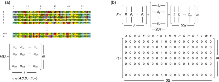
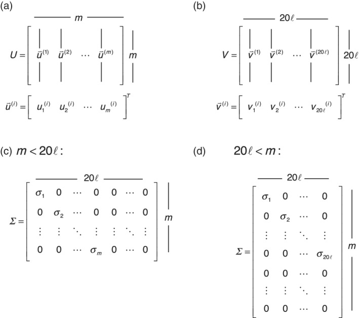
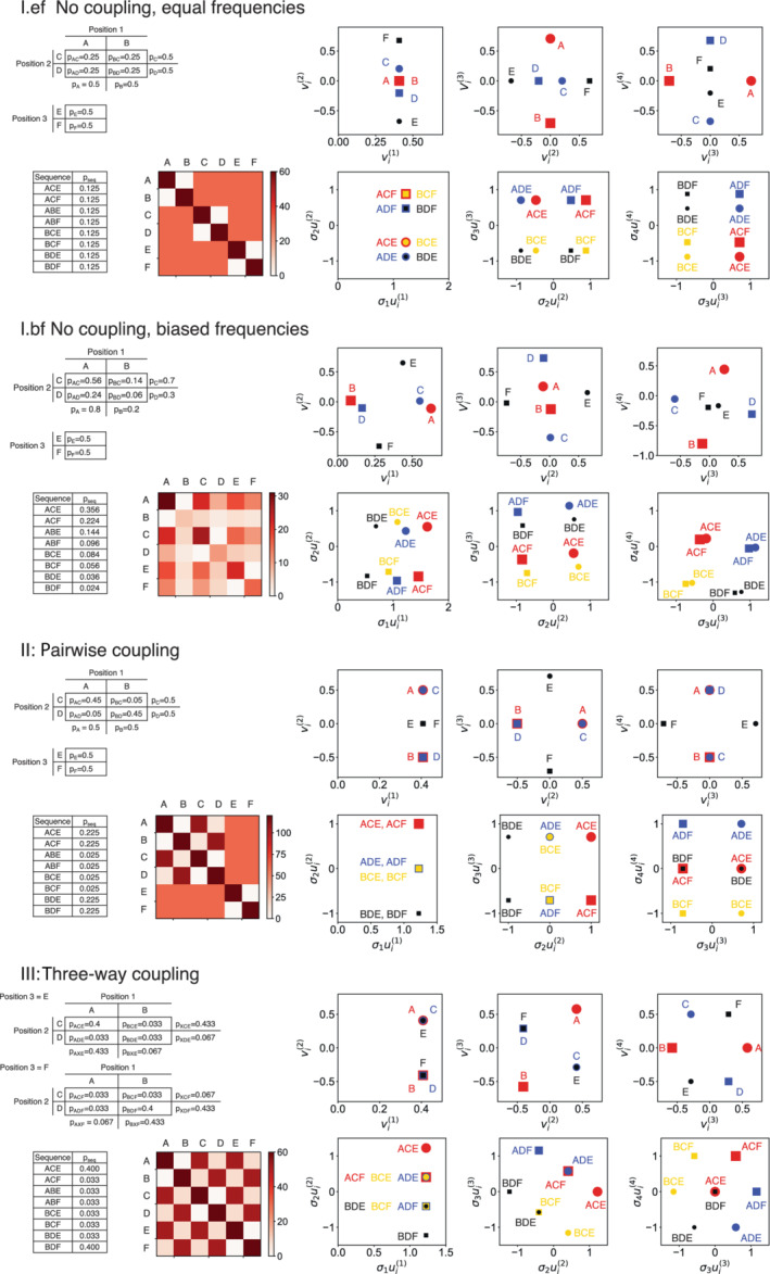
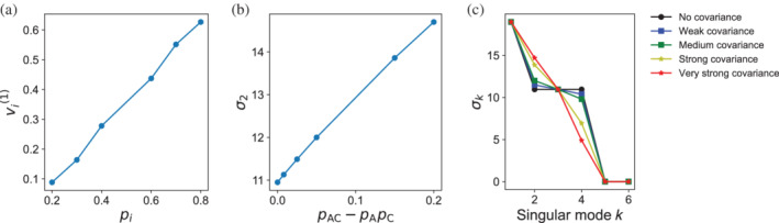
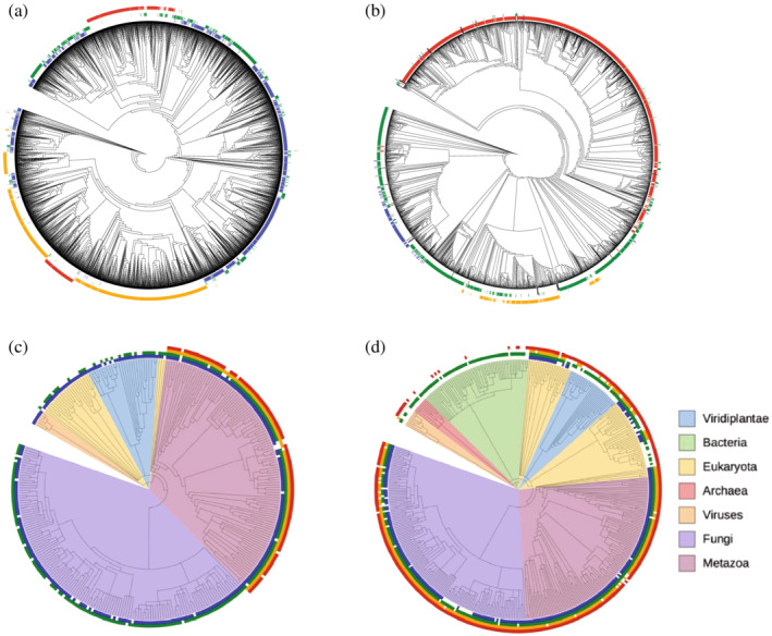
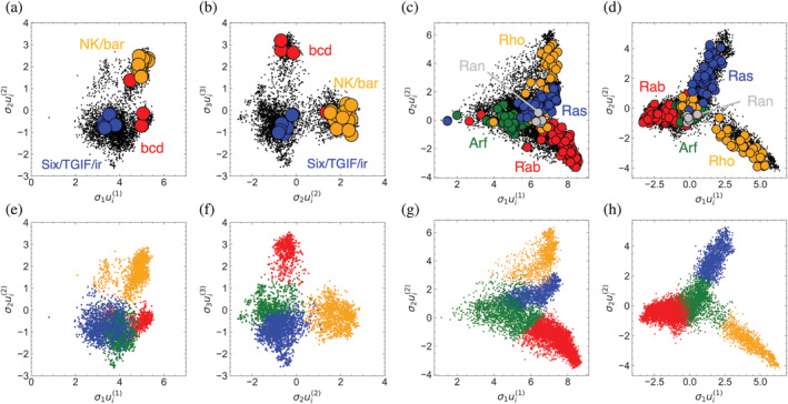
Singular value decomposition (SVD) of multiple sequence alignments (MSAs) is an important and rigorous method to identify subgroups of sequences within the MSA, and to extract consensus and covariance sequence features that define the alignment and distinguish the subgroups. This information can be correlated to structure, function, stability, and taxonomy. However, the mathematics of SVD is unfamiliar to many in the field of protein science. Here, we attempt to present an intuitive yet comprehensive description of SVD analysis of MSAs. We begin by describing the underlying mathematics of SVD in a way that is both rigorous and accessible. Next, we use SVD to analyze sequences generated with a simplified model in which the extent of sequence conservation and covariance between different positions is controlled, to show how conservation and covariance produce features in the decomposed coordinate system. We then use SVD to analyze alignments of two protein families, the homeodomain and the Ras superfamilies. Both families show clear evidence of sequence clustering when projected into singular value space. We use k-means clustering to group MSA sequences into specific clusters, show how the residues that distinguish these clusters can be identified, and show how these clusters can be related to taxonomy and function. We end by providing a description a set of Python scripts that can be used for SVD analysis of MSAs, displaying results, and identifying and analyzing sequence clusters. These scripts are freely available on GitHub.

Keywords: bioinformatics; protein design; singular value decomposition; taxonomy.

FIGURE 1

Matrix representation of a multiple sequence alignment. (a) A multiple sequence alignment (top) of $m$ sequences of length $\ell$= 56 residues. The alignment can be thought of as a matrix of $m$ rows and $\ell$ columns, where each matrix element is one of the 20 amino acids ($\alpha$) along with the gap residue. (b) A binary representation F of the MSA matrix, where each position is represented by an $m$ by $20$ block matrix $P$. Each column of the block matrix corresponds to one of the 20 amino acids at a given position. Each row in the block matrix corresponds to a position in a particular sequence in the MSA, and contains a one in the column corresponding to the amino acid at that position and zeros in all other columns. If a sequence $i$ contains a gap at a particular position, row $i$ of the corresponding block matrix contains 20 zeros. F can be viewed as (i) a collection of m binary sequence row vectors ${\stackrel{\rightharpoonup }{s}}_i$, each of length $20\ell$ or (ii) a collection of $20\ell$ binary residue column vectors ${\stackrel{\rightharpoonup }{r}}_i$, each of length $m.$

FIGURE 2

Features of the matrices in singular value decomposition. (a,b) Sequence and residue eigenvector matrices U and V , along with the i ^th singular vector for each matrix. (c, d) Singular value matrices. In (c), the number of rows (sequences) is small compared to the binary encoding of the sequence length (20 times residues plus gap positions in the MSA). In (d), the number of rows (sequences) is large compared to the binary sequence length.

FIGURE 3

The effects of bias and coupling on SVD coordinates of residues and sequences. A simple three‐position sequence with two residues at each position (A, B at position 1, C, D at position 2, and E, F at position 3) is used to generate MSAs with varying degrees of sequence bias and coupling. In model I.ef (top), the six residues have equal overall frequencies (of 0.5). In model I.bf (upper middle), the six residues occur with different frequencies, as given by the marginal probabilities (e.g., p _A) in the table on the lower left. In both versions of model I, residue frequencies are independent of each other, such that residue pair probabilities are given by the product of the marginal probabilities. In model II (lower middle), there is pairwise covariance between positions 1 and 2, but position 3 is independent of the other two. In model III (bottom), there is three‐way covariance between positions 1, 2, and 3. For each model, joint and marginal probabilities and probabilities for the eight different sequences are given in the upper left, residue pair count matrices ($D=F^{T}F$) are shown in the lower left, residue $v_i^{\left(k\right)}$ values along singular coordinates 1–4 are shown in the upper right, and sequence ${\sigma }_k{u}_i^{\left(k\right)}$ values along singular coordinates 1–4 are shown in the lower right.

FIGURE 4

The effects of sequence bias and correlation on residue coordinates and singular values. (a) For model I.bf, where residues at the same position have different probabilities (Figure 3), the residue $v_i^{\left(1\right)}$ values along the first singular coordinate are correlated with the residue probability. (b) for model II, where there is a pairwise correlation between residues A and C at positions 1 and 2, the singular value ${\sigma }_2$ is correlated with covariance between residues A and C (likewise for residues B and D, not shown). (c) For model II, as the strength of the pairwise covariance increases, ${\sigma }_2$ increases at the expense of ${\sigma }_4$, indicating that when correlation increases, fewer components are needed in the SVD.

FIGURE 5

The coordinates each sequence in SVD space is the sum of the coordinates of its residues. Singular value decomposition of a three‐position, six‐residue model described above was used to generate sequence coordinates ${\sigma }_k{u}_i^{\left(k\right)}$ and residue coordinates $v_j^{\left(k\right)}$. In this model, there is sequence bias at each position (p _A = 0.8, p _B = 0.2, p _C = 0.7, p _D = 0.3, p _E = 0.6, p _F = 0.4) as well as pairwise correlation between positions 1 and 2 (p _AC = 0.65, p _AD = 0.15, p _BC = 0.05, p _BD = 0.15). Each of the six residues are plotted in the first and second singular dimensions ($v_i^{\left(1\right)}$, $v_i^{\left(2\right)}$; circles and dashed arrows) along with one sequence (${\sigma }_1{u}_i^{\left(1\right)}$, ${\sigma }_2{u}_i^{\left(2\right)}$; plus sign) per panel. SVD, singular value decomposition

FIGURE 6

Singular values for homeodomain and Ras. (a,c) Singular values and (b,d) cumulative singular values for homeodomain (a,b) and Ras (c,d) are shown in black bars. Red bars are singular values for an MSA where residues in each column is randomly shuffled, eliminating sequence covariance. Blue bars are singular values for an 𝐹‐matrix where each column is randomly shuffled. In total, the singular values sum to 9,646 and 37,273 for HD and Ras, respectively. MSA, multiple sequence alignment

FIGURE 7

The sequence spaces of HD and Ras generated by SVD. Each point corresponds to a single HD (a,b) or Ras superfamily sequence (c,d) from the MSAs analyzed by SVD. Pink stars are consensus sequences derived from the entire MSA. k‐Means clustering was performed on ${\sigma }_1{u}_i^{\left(1\right)}$, ${\sigma }_2{u}_i^{\left(2\right)}$, and ${\sigma }_3{u}_i^{\left(3\right)}$ values to assign sequences to one of four clusters (colored red, blue, orange, and green). To visualize the 3D plots from different angles, see Videos S1 and S2. MSA, multiple sequence alignment; SVD, singular value decomposition

FIGURE 8

Residue distributions in SVD sequence space. Each point corresponds to one of the $20\ell$ residues of the HD (a,b) or Ras (c,d) MSAs. Values are the elements of the residue eigenvectors (Equation 5). Although scaling these values by their corresponding values would weigh the relative contribution of residues to the sequence alignment, plotting unscaled values gives the direct contribution of each residue in a sequence to the corresponding value (Figure 5). Colored points indicate residues that have frequencies within a k‐means cluster enriched by 0.4 or greater compared to out‐of‐cluster residue frequencies, and represent a sequence signature for that particular cluster. Colors are the same as in Figure 7. To visualize the 3D plots from different angles, see Videos S3 and S4. MSA, multiple sequence alignment; SVD, singular value decomposition

FIGURE 9

Phylogenetic trees and their relation to SVD clusters. (a,b) Sequence trees of sequences in the HD and Ras MSAs, respectively. (c,d) Species trees of sequences in the HD and Ras MSAs, respectively. Colored marks on the outside of each tree indicate cluster identities using the color scheme in Figure 7. For the species trees, color wedges on the inside indicate major taxa. Sequence trees were generated in MAFFT using default settings. Species trees were generated from PhyloT (https://phylot.biobyte.de/), using the UniProt IDs associated with each sequence in Pfam. Note that there are fewer sequences on the species trees (310 and 430 for HD and Ras, respectively) than on the sequence trees (4,995 and 10,265 for HD and Ras, respectively) because only sequences from organisms with unique UniProt IDs can be depicted. Trees were rendered using iTOL. MSA, multiple sequence alignment; SVD, singular value decomposition

FIGURE 10

Mapping functional features into SVD space. Projection of sequences with known HD DNA binding specificities (a,b) and Ras‐family specializations (c,d) into SVD space. Projected sequences are colored according to clusters from Figure 7, which are reproduced (e–h) for comparison, and colored black in the projections to contrast the projected sequences. For both protein families, projected sequences segregate to a particular cluster, indicating that these clusters represent specific functional groups. SVD, singular value decomposition

References

1. Ekeberg M, Lövkvist C, Lan Y, Weigt M, Aurell E. Improved contact prediction in proteins: Using pseudolikelihoods to infer Potts models. Phys Rev E Stat Nonlin Soft Matter Phys. 2013;87(1):012707. 10.1103/PhysRevE.87.012707. - DOI - PubMed
1. Morcos F, Pagnani A, Lunt B, et al. Direct‐coupling analysis of residue coevolution captures native contacts across many protein families. Proc Natl Acad Sci U S A. 2011;108(49):E1293–E1301. 10.1073/pnas.1111471108. - DOI - PMC - PubMed
1. Russ WP, Figliuzzi M, Stocker C, et al. An evolution‐based model for designing Chorismate mutase enzymes. Science. 2020;369(6502):440–445. 10.1126/science.aba3304. - DOI - PubMed
1. Halabi N, Rivoire O, Leibler S, Ranganathan R. Protein sectors: Evolutionary units of three‐dimensional structure. Cell. 2009;138(4):774–786. 10.1016/j.cell.2009.07.038. - DOI - PMC - PubMed
1. Rivoire O, Reynolds KA, Ranganathan R. Evolution‐based functional decomposition of proteins. PLoS Comput Biol. 2016;12(6):e1004817. 10.1371/journal.pcbi.1004817. - DOI - PMC - PubMed
Publication types