. 2023 Apr;7(4):520-532.
doi: 10.1038/s41551-022-00941-y. Epub 2022 Oct 3.

Ultraflexible electrode arrays for months-long high-density electrophysiological mapping of thousands of neurons in rodents

Affiliations

Ultraflexible electrode arrays for months-long high-density electrophysiological mapping of thousands of neurons in rodents

Zhengtuo Zhao et al. Nat Biomed Eng. 2023 Apr.

Abstract

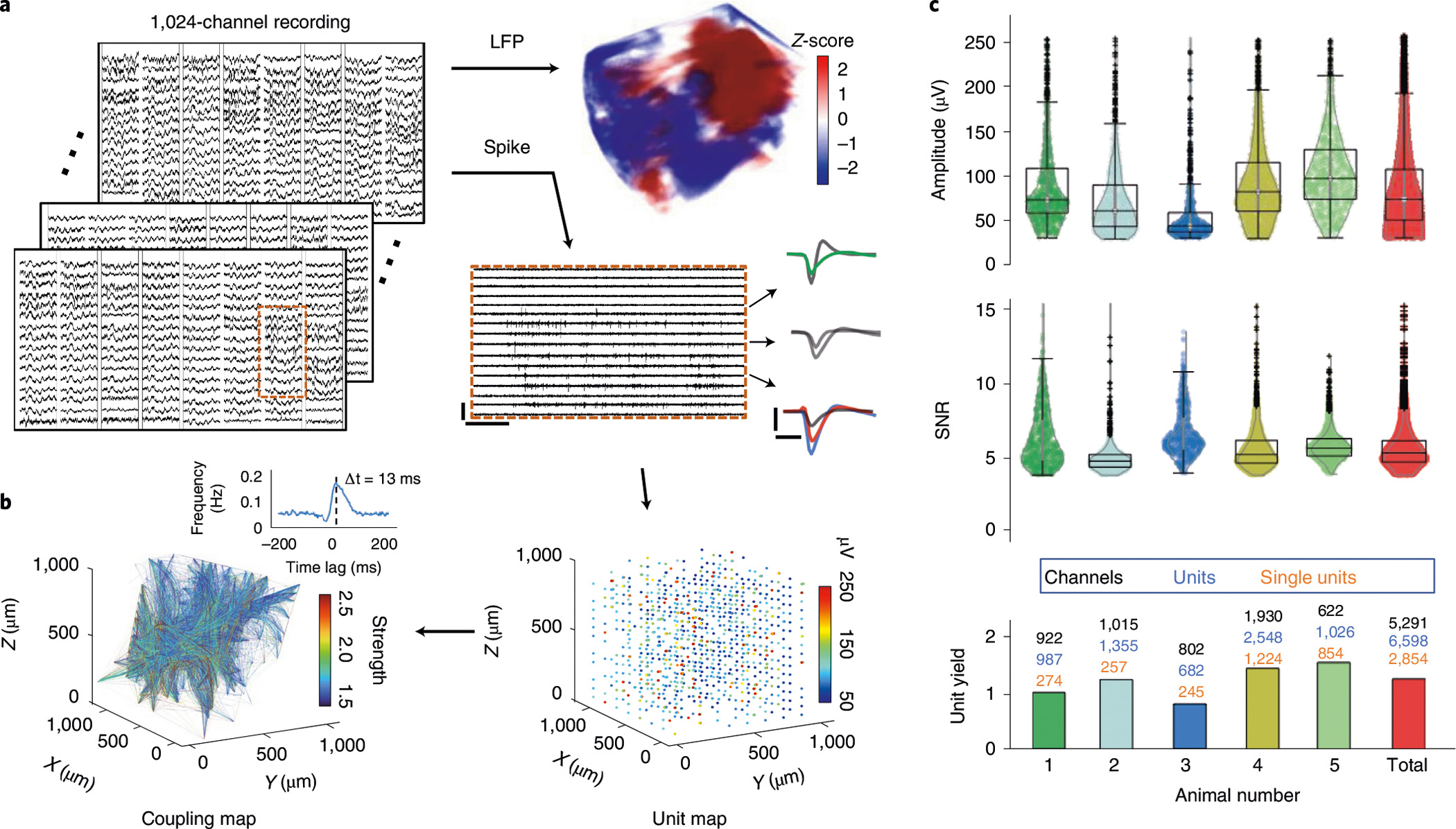
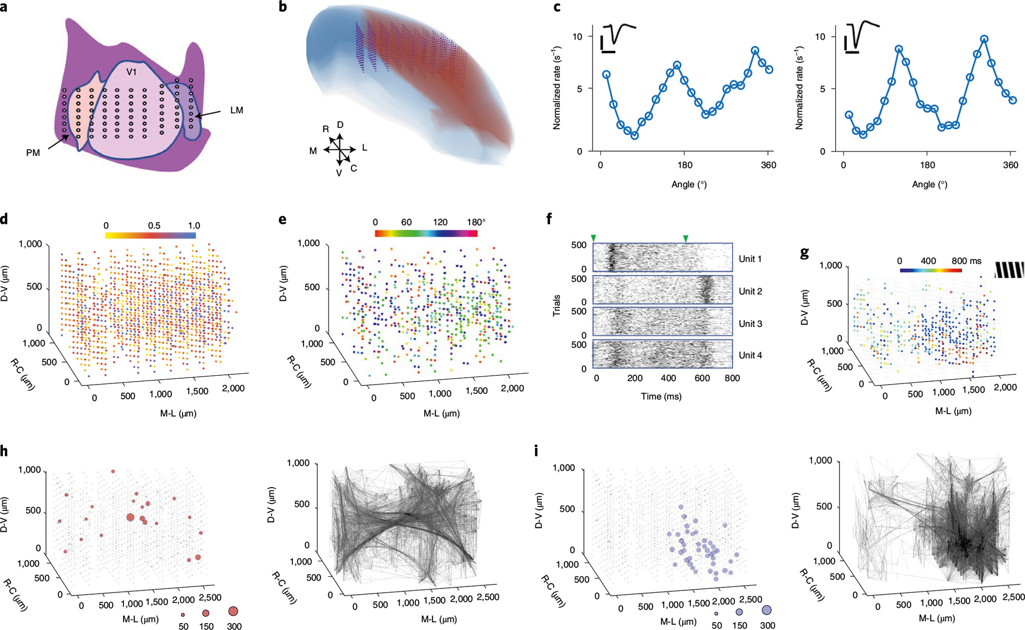
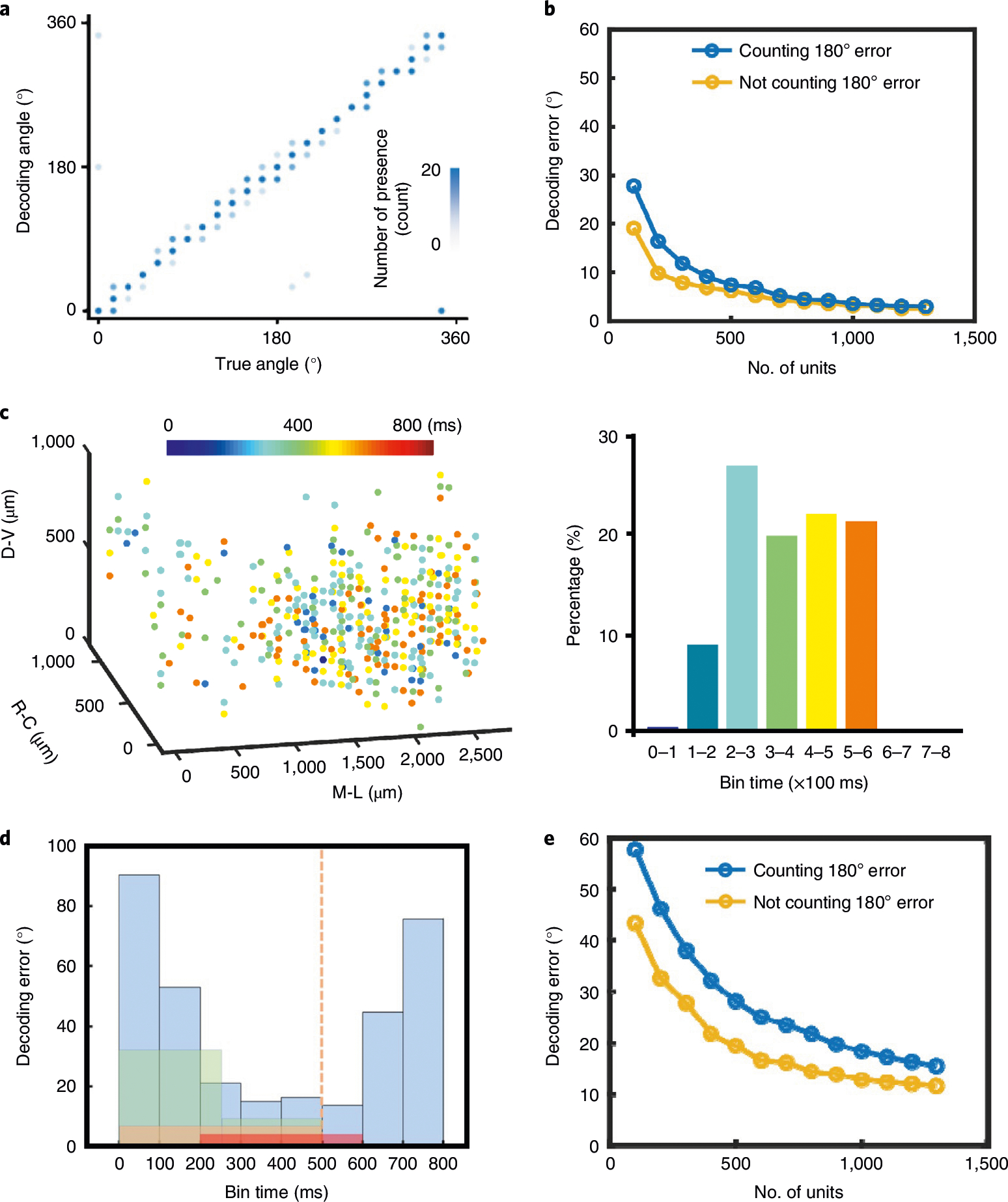
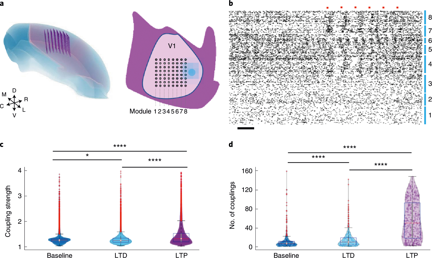
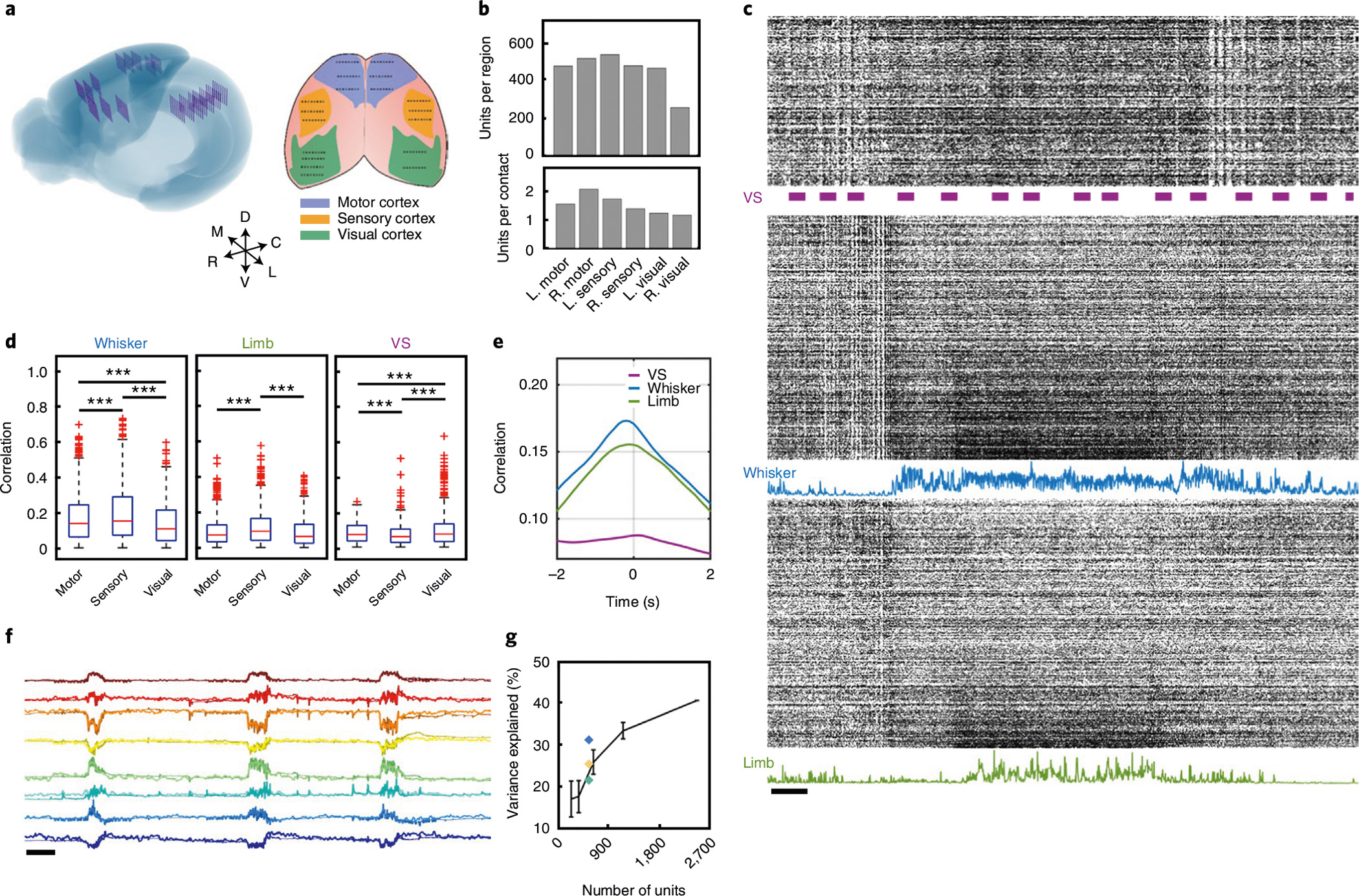
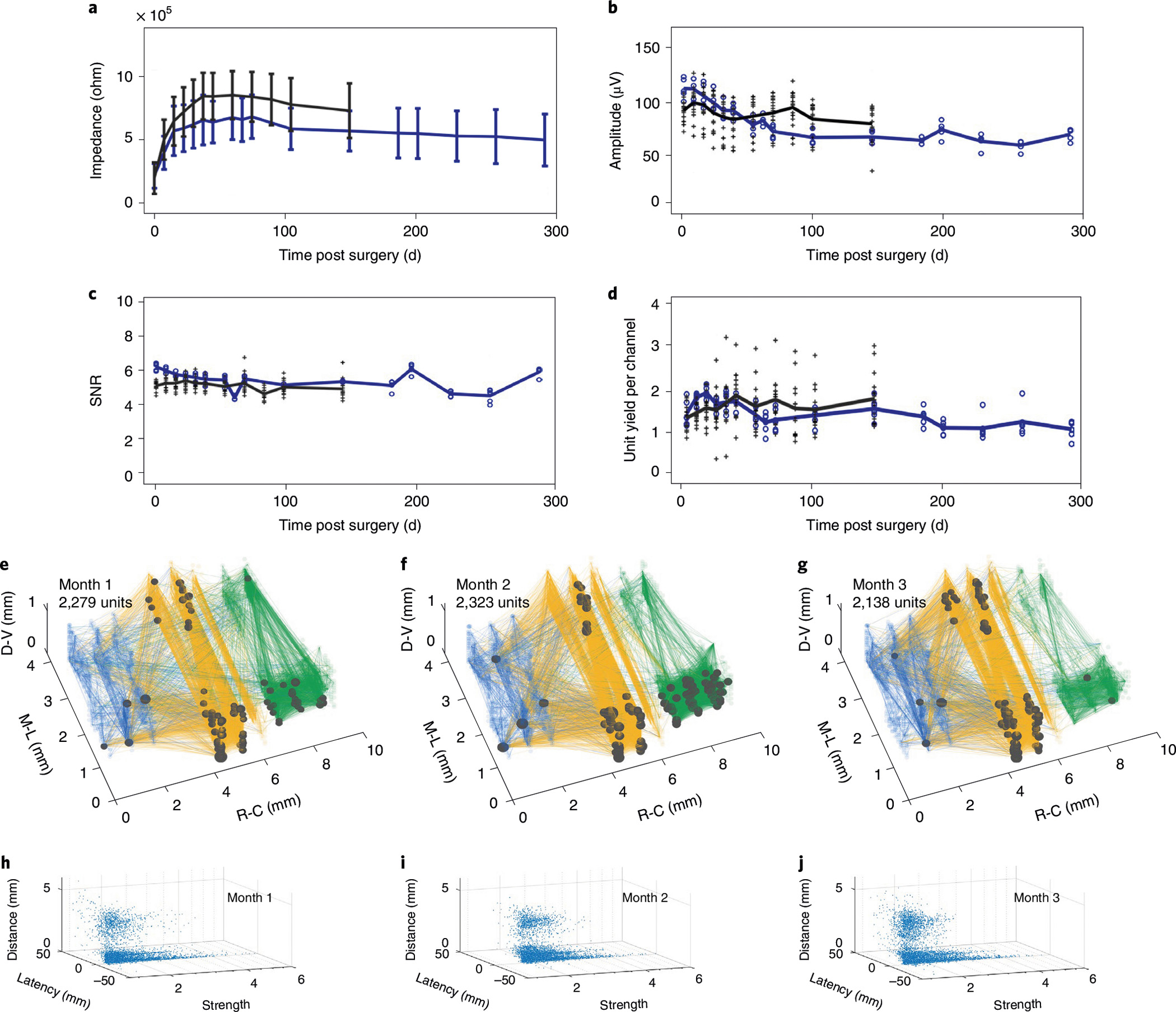
Penetrating flexible electrode arrays can simultaneously record thousands of individual neurons in the brains of live animals. However, it has been challenging to spatially map and longitudinally monitor the dynamics of large three-dimensional neural networks. Here we show that optimized ultraflexible electrode arrays distributed across multiple cortical regions in head-fixed mice and in freely moving rats allow for months-long stable electrophysiological recording of several thousand neurons at densities of about 1,000 neural units per cubic millimetre. The chronic recordings enhanced decoding accuracy during optogenetic stimulation and enabled the detection of strongly coupled neuron pairs at the million-pair and millisecond scales, and thus the inference of patterns of directional information flow. Longitudinal and volumetric measurements of neural couplings may facilitate the study of large-scale neural circuits.


Conflict of interest statement

Competing interests

C.X., L.L. and Z.Z. are co-inventors on a patent filed by The University of Texas (WO2019051163A1, 14 March 2019) on the ultraflexible neural electrode technology described in this study. L. F., L.L. and C.X. hold equity ownership in Neuralthread Inc., an entity that is licensing this technology. All other authors declare no competing interests.

Figures

Extended Data Fig. 1 |
Extended Data Fig. 1 |. Immunohistochemistry analysis showing the tissue-NET interface at a high implantation density.
One mouse was implanted in visual cortex with 10 type-I NET modules, at inter-shank spacings of 150 μm and inter-module spacings of 250 μm. Fluorescent (a) and brightfield (b) microscopy show no observable scarring in the implanted regions. Neuron: red; NETs: yellow. (c), We counted numbers of neurons in seven randomly-chosen 200-μm-diameter regions centering around NETs (yellow circled regions as an example) and five 200-μm-diameter randomly-chosen regions away from NETs (cyan circled regions as an example). We found no significant difference between the two groups using unpaired T test, p = 0.275 (d), suggesting no significant neuronal loss induced by dense NET implants. These results are consistent with our prior studies using single or few NETs (10, 13). Scalebars: 250 μm (a and b) and 50 μm (c).
Extended Data Fig. 2 |
Extended Data Fig. 2 |. Example recording performances of type-II (A) and –III (B) NET electrode designs.
These two designs offer high electrode density that allows for the recording of individual neurons by multiple channels and therefore perform better in single unit isolation. Color code corresponds to the location of the recording sites. Each dashed box outlines the waveforms of a single unit recorded on the corresponding sites. Scale bars: 100 μV (vertical) and 2 ms (horizontal).
Extended Data Fig. 3 |
Extended Data Fig. 3 |. Modular recording system interfacing with NETs.
(a), A ready-to-implant 128-channel NET module connected to a flexible printed circuit (FPC). Left panel shows the NET module and ball grid array (BGA) through which the connection to FPC was made. Right panel shows that individual NET shanks was attached to tungsten microwires for implantation. (b), Photo of a 128-channal stackable headstage connected to NET through an FPC. (c), Photo of a 1024-channel system composed of eight stackable modules. (d), Photo of a free-moving rat carrying a 1024-channel NET array and stackable headstages as shown in c. 3D printed case enclosed all headstages.
Fig. 1 |
Fig. 1 |. Overview of the large-scale modular NET technology.
a, Left: a micro-CT scan of an implanted NET array in a rat brain consisting of 8 128-channel modules (1,024 channels in total) at high 3D density. The purple cube highlights the NET array. Right: schematics of the 3D NET array embedded in cortical tissues. b, Images of the three types of NET arrays used in the study. c, Photos of a 128-channel type-I NET module. Red dotted box highlights the released front end. Inset: 8-shank, 128-channel flexible section immersed in water. d, Schematics showing assembled NET modules (each containing 8 × 16 intracortical recording sites) implanted sequentially into the brain using a pair of stereotaxic micromanipulators, one module at a time. e, A micro-CT scan showing the volumetric distribution of an 8 × 8 × 16 (1,024-channel) NET array in a mouse visual cortex. The targeted module-to-module spacing is 150 μm. Scale bars, 50 μm (b), 500 μm (c) and 500 μm (e).
Fig. 2 |
Fig. 2 |. Overview of the recording performance.
a, Representative recordings from 1,024 channels in an animal (#1 in c) showing both LFP (bandpass filtered at (8 12) Hz) and spikes (high-pass filtered at 300 Hz). Scale bars, 250 μV (vertical) and 0.3 s (horizontal). Typical waveforms are depicted. Scale bars, 100 μV (vertical) and 1 ms (horizontal). b, Volumetric recording enables reconstruction of unit location (right) and mapping of pairwise correlation (left). The amplitude of units and the coupling strength are colour coded. Inset: a representative cross-correlogram showing the detection of temporal bias at the millisecond resolution. c, Distribution of unit amplitude, SNR and unit yields of n = 5 implanted animals. The average of all units is shown in the last column. All units are shown in the violin plots.
Fig. 3 |
Fig. 3 |. Volumetric high-density mapping of the visual cortex in an awake head-fixed mouse.
a, Schematic representation of the targeted implantation location in the visual cortex. LM, lateromedial area; V1, primary visual cortex; PM, posteromedial area. Each dot represents a 16-channel shank. b, Reconstruction of expected locations of all 8 × 10 recording shanks (1,280 channels). Blue, neocortex of right hemisphere; red, visual area; purple, NET arrays. D, V, R, C, M and L denote the orientations of dorsal, ventral, anterior, posterior, medial and lateral, respectively. c, Two sorted units recorded by the same contact in V1 showing distinct orientation tuning curves. Inset: unit waveforms. Scale bars, 1 ms (horizontal) and 100 μV (vertical). d, Colour-coded OSI for all recorded units (1,355 in total). All units are individually plotted as a sphere superimposed on the closest contact site. e, Preferred angle of grating for units with OSI > 0.5. f, Spike raster of 500 trials from representative units highlighting different temporal responses to grating stimuli. Triangles mark the start and end of the gratings. g, The peak firing time from the most active 30% of units under a stimulus of 165° drifting grating (shown in the upper right inset). h,i, Spatial distribution of the super nodes (left) and the strong couplings (right) without (h) and with (i) visual stimulation. The diameter of the circles is scaled to the number of couplings made at each node.
Fig. 4 |
Fig. 4 |. Visual decoding using large-scale neural recordings.
a, True versus decoded orientation of the drifting gratings. Contrast is scaled to the number of presence. b, Scaling of the mean decoding error with the number of recorded units using the time segment of 200–600 ms and 40 training trials. Stimuli were presented in the interval 0–500 ms. Decoding errors were computed in two ways: counting or not counting the 180° difference in the angles of drifting gratings. c, Spatiotemporal distribution of the units with the top 30% prediction power. Colours code the time at their maximum prediction power. Bars (right) present their population percentage. d, Mean decoding error as a function of selected time segment used for training. Colours mark different binning methods. Blue, every 100 ms; green, 0–250 ms and 250–500 ms; orange, 1–500 ms; red, 200–600 ms. The orange dashed line denotes the finish of visual stimulation. e, Scaling of the decoding error with the number of recorded units using the period of 300–400 ms and 40 training trials.
Fig. 5 |
Fig. 5 |. Simultaneous volumetric recording and optogenetic stimulation.
a, Schematic showing the targeted locations of the 8 × 8 × 16 recording sites in 3D (left), and the surface implantation locations for NET shanks (8 × 8) and the optical fibre (filled dot) in V1 (right). b, Spike raster of all 686 units recorded. Numbers mark the recording modules as in a. Orange dots mark the presence of optical stimulation. Scale bar, 0.1 s. c,d, Distribution of the couplings and nodes at baseline (blue), after optical LTD (cyan) and LTP (purple) protocols. Boxplots show the median, upper and lower 25%, and outliers. All data are shown in the violin plots. *P < 0.05, **P < 0.01, ****P < 0.0001, unpaired two-sided t-test, Bonferroni corrected.
Fig. 6 |
Fig. 6 |. Large-scale distributed recording in awake head-fixed mice and behaviour decoding.
a, Left: schematic showing reconstructed locations of all 144 recording shanks across the neocortex of mouse brain. Right: schematic representation of the surface implantation location with target brain region colour coded, each dot representing a 16-channel shank. b, Quantification of unit yield across six brain regions in a typical recording session. c, Representative spike raster of the 2,548 units recorded from the NET array. Three segments depict the units in the visual (top), sensory (middle) and motor (bottom) cortices. Bars mark the presence of visual stimuli. Blue and green curves plot the magnitude of the whisker deflection and limb motion, respectively. Scale bar, 1 s. d, Boxplots (median, upper and lower 25%, and outliers) showing the correlation between neural activity and three behavioural markers: whisker motion (left), limb motion (middle) and the presence of visual stimuli (right). Unpaired two-sided t-test, ***P < 0.001, Bonferroni corrected. e, Mean correlation of spike activity of all units and three biomarkers as a function of time latency. f, Prediction of eight latent behavioural states extracted from the face video with neural activity. Darker colours mark the real traces, and lighter colours mark the predicted traces. Scale bar, 10 s. g, Prediction performance (mean ± s.d., n = 5) as a function of brain regions used for decoding. Blue, motor area; yellow, sensory area; green, visual area; black, scaling of the prediction performance with the number of recorded units randomly selected from all regions.
Fig. 7 |
Fig. 7 |. Chronic stability of large-scale recordings by NETs, and evaluation of network stability over time.
ad, Performance and stability of unit recordings from 21 128-channel modules over time. The averaged values of impedance (a), peak-to-valley amplitude (b), SNR (c) and single- and multi-unit yield (d) remained stable for the experimental duration, except for the initial changes within 60 days after implantation. Each cross and dot presents the module-averaged values from 16 modules that were tracked for 145 days and from the other 5 modules that were tracked for 290 days, respectively. Black and blue lines depict the average values of all 16 and 5 modules, respectively. Error bars in a denote s.d. eg, Cortical network stability over 3 months demonstrated by the spatial distribution of the strong couplings (lines) and super nodes (dots) under visual stimuli. The size of the dots indicates the number of couplings from the node. Measurement time and total unit number are indicated. hj, Distribution of the coupling strength, latency and separation between the pairs under visual stimulation at 1 (h), 2 (i) and 3 (j) months post implantation, respectively.

Comment in

Similar articles

Cited by

References

    1. Braitenberg V & Schüz A Anatomy of the Cortex: Statistics and Geometry (Springer, 1991).
    1. Kleinfeld D et al. Can one concurrently record electrical spikes from every neuron in a mammalian brain? Neuron 103, 1005–1015 (2019). - PMC - PubMed
    1. Marblestone AH et al. Physical principles for scalable neural recording. Front. Comput. Neurosci. 7, 137 (2013). - PMC - PubMed
    1. Chen TW et al. Ultrasensitive fluorescent proteins for imaging neuronal activity. Nature 499, 295–300 (2013). - PMC - PubMed
    1. Adam Y et al. All-optical electrophysiology reveals brain-state dependent changes in hippocampal subthreshold dynamics and excitability. Nature 569, 413 (2019). - PMC - PubMed

Publication types