Concentration fluctuations in growing and dividing cells: Insights into the emergence of concentration homeostasis

Abstract

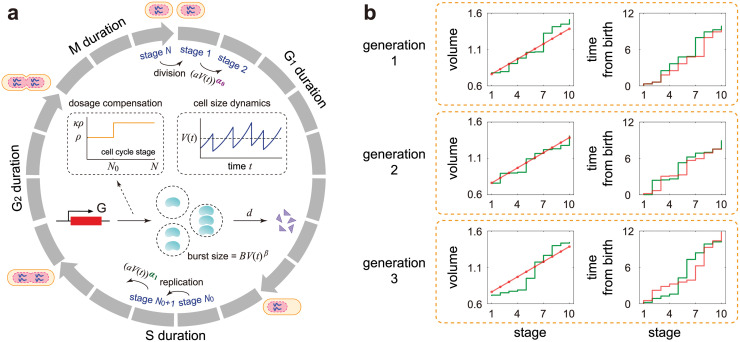
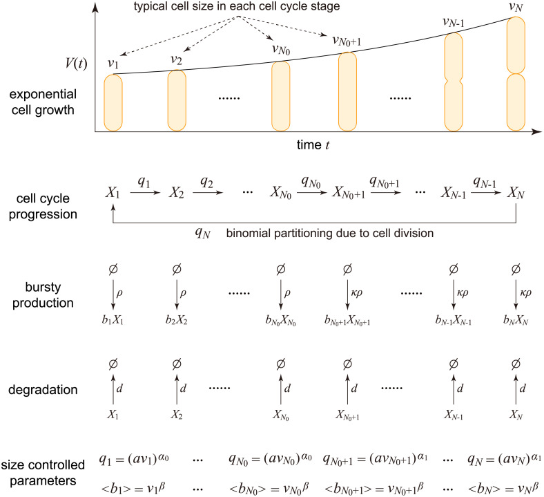
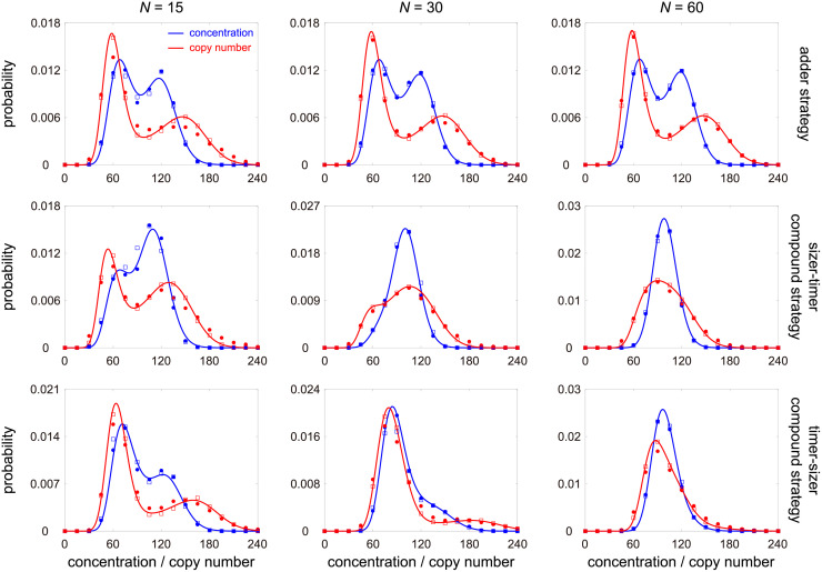
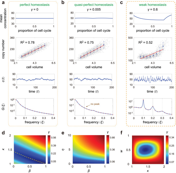
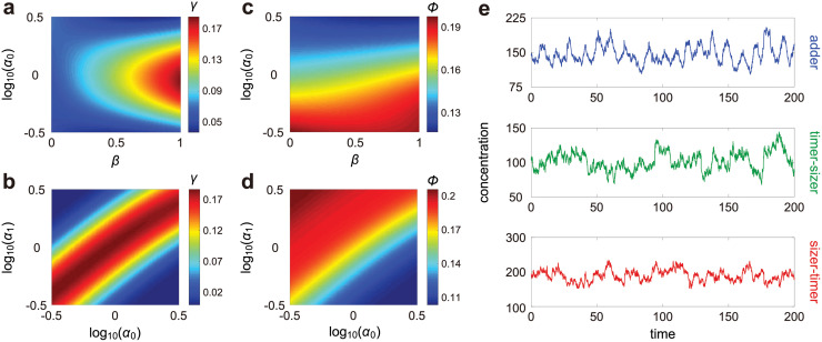
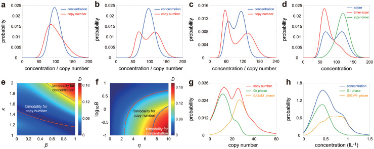
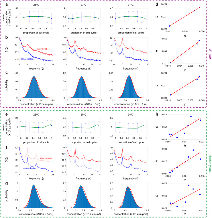
Intracellular reaction rates depend on concentrations and hence their levels are often regulated. However classical models of stochastic gene expression lack a cell size description and cannot be used to predict noise in concentrations. Here, we construct a model of gene product dynamics that includes a description of cell growth, cell division, size-dependent gene expression, gene dosage compensation, and size control mechanisms that can vary with the cell cycle phase. We obtain expressions for the approximate distributions and power spectra of concentration fluctuations which lead to insight into the emergence of concentration homeostasis. We find that (i) the conditions necessary to suppress cell division-induced concentration oscillations are difficult to achieve; (ii) mRNA concentration and number distributions can have different number of modes; (iii) two-layer size control strategies such as sizer-timer or adder-timer are ideal because they maintain constant mean concentrations whilst minimising concentration noise; (iv) accurate concentration homeostasis requires a fine tuning of dosage compensation, replication timing, and size-dependent gene expression; (v) deviations from perfect concentration homeostasis show up as deviations of the concentration distribution from a gamma distribution. Some of these predictions are confirmed using data for E. coli, fission yeast, and budding yeast.

Fig 1. Model and its mean-field approximation.

A: A detailed stochastic model with both cell size and gene expression descriptions. The model consists of N effective cell cycle stages, gene replication at stage N₀, cell division at stage N, bursty production of the gene product, and degradation of the gene product. The growth of cell volume is assumed to be exponential and gene dosage compensation is induced by a change in the burst frequency at replication from ρ to κρ with κ ∈ [1, 2) (see inset graphs). Both the transition rates between stages and the mean burst size depend on cell size in a power law form due to size homeostasis and balanced (or non-balanced) biosynthesis, respectively. The model also considers two-layer cell-size control with its strength varying from α₀ to α₁ upon replication. B: Schematics of the changes in cell volume and time from birth as a function of cell cycle stage k for the first three generations in the case of N = 10 and α₀ = α₁ = 1. In the full model (green curve), the gene expression dynamics is coupled with the following two types of fluctuations: noise in cell volume at each stage and noise in the time interval between two stages. The reduced model (red curve) ignores the former type of fluctuations by applying a mean-field approximation while retaining the latter type of fluctuations. Note that when α₀ = α₁ = 1, it follows from Eq (3) that the mean cell volume at stage k is v_k = v₁ + (k − 1)M₀/N₀, which linearly depends on k. The red dots in the stage-volume plot show the dependence of v_k on k and the joining of these dots by a straight red line is simply a guide to the eye. The reduced model approximates the full model excellently when N is sufficiently large.

Fig 2. Reduced model obtained by making the mean-field approximation of cell size dynamics.

Here X_k denotes the gene product at stage k and b_k denotes the burst size at stage k. Moreover, v_k is the typical cell size at stage k, B_k is the mean burst size at stage k, and q_k is the typical transition rate from stage k to the next.

Fig 3. Comparison between the full and mean-field models under different choices of N and different size control strategies.

The blue (red) dots show the simulated concentration (copy number) distribution for the full model obtained from the stochastic simulation algorithm (SSA). The blue (red) squares show the simulated concentration (copy number) distribution for the mean-field model obtained from SSA. The blue (red) curve shows the analytical approximate concentration (copy number) distribution given in Eq (8) (Eq (15)). The full and mean-field models are in good agreement when N ≥ 15 and they become almost indistinguishable when N ≥ 30. Moreover, the analytical solution performs well when N ≥ 15 and perform excellently when N ≥ 30. The model parameters are chosen as N₀ = 0.4N, B = 1, β = 0, κ = 2, d = 1, η = 10, where η = d/f is the ratio of the degradation rate to cell cycle frequency. The growth rate g is determined so that f = 0.1. The parameters ρ and a are chosen so that the mean gene product number 〈n〉 = 100 and the mean cell volume 〈V〉 = 1. The strengths of size control are chosen as α₀ = α₁ = 1 for the upper panel, α₀ = 2, α₁ = 0.5 for the middle panel, and α₀ = 0.5, α₁ = 2 for the lower panel. When performing SSA, the maximum simulation time for each lineage is chosen to be 10⁵. To deal with the time-dependent propensities in the full model, we use the numerical algorithm described in [, Sec. 5].

Fig 4. Concentration homeostasis and its relation to concentration oscillations.

A: Perfect homeostasis. The first row shows the mean concentration μ_k at cell cycle stage k versus the proportion of cell cycle before stage k, which can be computed explicitly as w_k = log₂(v_k/v₁). The second row shows the scatter plot of molecule number versus cell volume obtained from SSA. Here data are sorted into 8 bins according to cell volume, and the mean and variance of molecule numbers within each bin are shown by the blue dot and the error bar. The red curve is the regression line for the scatter plot. The third row shows typical time traces of concentrations, where c(t) denotes the concentration at time t for a single cell lineage. The fourth row shows the theoretical (blue curve) and simulated (red circles) power spectra of concentration fluctuations. The theoretical spectrum is computed from Eq (9), while the simulated spectrum is obtained by means of the Wiener-Khinchin theorem, which states that $G\left(\xi \right)={\text{lim}}_{T\to \infty }\langle |{\widehat{c}}_T\left(\xi \right){|}^2\rangle /T$, where ${\widehat{c}}_T\left(\xi \right)={\int }_0^{T}c\left(t\right)e^{-2\pi i\xi t}dt$ is the truncated Fourier transform of a single concentration trajectory over the interval [0, T] and the angled brackets denote the ensemble average over trajectories. The vertical lines show the cell cycle frequency f and its harmonics. B: Same as A but for quasi-perfect homeostasis. C: Same as A but for weak homeostasis. D: Heat plot of γ (the accuracy of concentration homeostasis) versus β (the degree of balanced biosynthesis) and κ (the strength of dosage compensation) when replication occurs halfway through the cell cycle (w = 0.5). The yellow dashed line shows the exponential curve $\kappa ={\sqrt{2}}^{1-\beta }$, around which homeostasis is accurate. E: Heat plot of γ versus β and η (the stability of the gene product) when there is no dosage compensation (κ = 2). Stable gene products give rise to more accurate homeostasis than unstable ones. F: Heat plot of γ versus κ and w (the proportion of cell cycle before replication) when synthesis is non-balanced (β = 0). Homeostasis is the most accurate when $\kappa =\sqrt{2}$ and w = 0.5. See Section D in S1 Appendix for the technical details of this figure.

Fig 5. Influence of size control on concentration homeostasis and concentration noise.

A,B: Heat plot of γ (the accuracy of concentration homeostasis) versus β (the degree of balanced biosynthesis), α₀ (the strength of size control before replication), and α₁ (the strength of size control after replication). When synthesis is balanced (β = 1), concentration homeostasis is accurate when the cell applies different size control strategies before and after replication. Both the timer-sizer and sizer-timer compound strategies enhance the accuracy of homeostasis. C,D: Heat plot of ϕ (noise in concentration) versus β, α₀, and α₁. While the timer-sizer compound strategy leads to accurate concentration homeostasis, it results in large gene expression noise. The sizer-timer compound strategy both maintains homeostasis and reduces noise. The model parameters are chosen as N = 50, N₀ = 21, ρ = 4.7, B = 1, κ = 2, d = 0.4, η = 4 in A-D, α₁ = 1 in A,C, and β = 1 in B,D. The growth rate g is determined so that f = 0.1. The parameter a is chosen so that the mean cell volume 〈V〉 = 1. E: Typical time traces of concentration under three different size control strategies: adder (upper panel), timer-sizer (middle panel), and sizer-timer (lower panel). See Section E in S1 Appendix for the technical details of this figure.

Fig 6. Influence of model parameters on copy number and concentration distributions.

A-C: The copy number (red curve) and concentration (blue curve) distributions display different shapes under different choices of parameters. A Both distributions are unimodal. B The concentration distribution is unimodal while the copy number one is bimodal. C Both distributions are bimodal. D: Concentration distributions under three different size control strategies: adder (blue curve), timer-sizer (red curve), and sizer-timer (green curve). Two-layer control strategies lead to unimodal concentration distributions that are not far from gamma. E,F: Heat plot of the Hellinger distance D of the concentration distribution from its gamma approximation versus β (the degree of balanced biosynthesis), κ (the strength of dosage compensation), η (the stability of the gene product), and B (the mean burst size). The violet (blue) curve encloses the region for the copy number (concentration) distribution being bimodal. The bimodal region for the copy number distribution is much larger than that for the concentration distribution. G,H: The mRNA copy number (red curve) and concentration (blue curve) distributions for the HTB2 gene in budding yeast measured using smFISH. The green (yellow) curves show the distributions of cells in the G₁ (G₂-S-M) phase. No apparent dosage compensation was observed with the mean copy number (concentration) in G₂-S-M being 2.22 (1.66) times greater than that in G₁. The data shown are published in [92]. See Section F in S1 Appendix for the technical details of this figure.

Fig 7. Analysis of single-cell lineage data of concentration fluctuations in E. coli and fission yeast.

The data shown are published in [23, 96]. The E. coli data set contains the lineage measurements of both cell length and fluorescence intensity of a stable fluorescent protein at three different temperatures (25°C, 27°C, and 37°C). The fission yeast data set contains the lineage measurements of both cell area and fluorescence intensity of a stable fluorescent protein under seven different growth conditions (Edinburgh minimal medium (EMM) at 28°C, 30°C, 32°C, and 34°C and yeast extract medium (YE) at 28°C, 30°C, and 34°C). A: The change in the mean concentration across the cell cycle for E. coli under three growth conditions. Here, we divide each cell cycle into 50 pieces and compute the mean and standard deviation (see error bars) of all data points that fall into each piece. The CV squared of the mean concentrations of all pieces gives an estimate of ϕ_ext and the CV squared of the concentrations of all cells gives an estimate of ϕ, from which γ can be inferred. B: Power spectra of copy number (red curve) and concentration (blue curve) fluctuations under three growth conditions. C: Experimental concentration distributions (blue bars) and their gamma approximations (red curve) under three growth conditions. D: Scatter plots between γ (the accuracy of concentration homeostasis), H (the height of the off-zero peak of the power spectrum), and D (the Hellinger distance between the concentration distribution from its gamma approximation) under three growth conditions. E-H: Same as A-D but for fission yeast. Here E-G only show the three growth conditions for YE, while H shows the scatter plots between γ, H, and D under all seven growth conditions (for both EMM and YE). Both cell types show remarkable positive correlations between γ, H, and D.

References

1. Peccoud J, Ycart B. Markovian modeling of gene-product synthesis. Theor Popul Biol. 1995;48(2):222–234. doi: 10.1006/tpbi.1995.1027 - DOI
1. Shahrezaei V, Swain PS. Analytical distributions for stochastic gene expression. Proc Natl Acad Sci USA. 2008;105(45):17256–17261. doi: 10.1073/pnas.0803850105 - DOI - PMC - PubMed
1. Smith S, Grima R. Single-cell variability in multicellular organisms. Nat Commun. 2018;9(1):1–8. doi: 10.1038/s41467-017-02710-x - DOI - PMC - PubMed
1. Zenklusen D, Larson DR, Singer RH. Single-RNA counting reveals alternative modes of gene expression in yeast. Nat Struct Mol Biol. 2008;15(12):1263–1271. doi: 10.1038/nsmb.1514 - DOI - PMC - PubMed
1. Larsson AJ, Johnsson P, Hagemann-Jensen M, Hartmanis L, Faridani OR, Reinius B, et al.. Genomic encoding of transcriptional burst kinetics. Nature. 2019;565(7738):251–254. doi: 10.1038/s41586-018-0836-1 - DOI - PMC - PubMed
Publication types
LinkOut - more resources