EpiLPS: A fast and flexible Bayesian tool for estimation of the time-varying reproduction number

Abstract

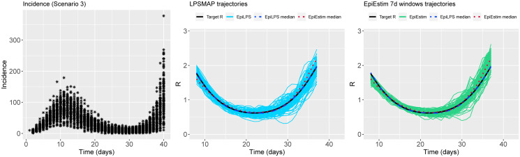
In infectious disease epidemiology, the instantaneous reproduction number [Formula: see text] is a time-varying parameter defined as the average number of secondary infections generated by an infected individual at time t. It is therefore a crucial epidemiological statistic that assists public health decision makers in the management of an epidemic. We present a new Bayesian tool (EpiLPS) for robust estimation of the time-varying reproduction number. The proposed methodology smooths the epidemic curve and allows to obtain (approximate) point estimates and credible intervals of [Formula: see text] by employing the renewal equation, using Bayesian P-splines coupled with Laplace approximations of the conditional posterior of the spline vector. Two alternative approaches for inference are presented: (1) an approach based on a maximum a posteriori argument for the model hyperparameters, delivering estimates of [Formula: see text] in only a few seconds; and (2) an approach based on a Markov chain Monte Carlo (MCMC) scheme with underlying Langevin dynamics for efficient sampling of the posterior target distribution. Case counts per unit of time are assumed to follow a negative binomial distribution to account for potential overdispersion in the data that would not be captured by a classic Poisson model. Furthermore, after smoothing the epidemic curve, a "plug-in'' estimate of the reproduction number can be obtained from the renewal equation yielding a closed form expression of [Formula: see text] as a function of the spline parameters. The approach is extremely fast and free of arbitrary smoothing assumptions. EpiLPS is applied on data of SARS-CoV-1 in Hong-Kong (2003), influenza A H1N1 (2009) in the USA and on the SARS-CoV-2 pandemic (2020-2021) for Belgium, Portugal, Denmark and France.

Fig 1

Illustration of smoothing windows of width ω to estimate ${\mathcal{R}}_t$ with EpiEstim. (a) Cori et al. (2013) [3] convention with sliding windows [t − ω; t], where ${\mathcal{R}}_t$ is reported at the end of the window. (b) Gostic et al. (2020) [2] recommendation with centered sliding windows [t − ω/2; t + ω/2], where ${\mathcal{R}}_t$ is reported at the midpoint of the window. Under the midpoint rule, ${\mathcal{R}}_t$ estimates for the last ω/2 time units are unavailable ∅.

Fig 2

(Left) Simulated incidence data for Scenario 2. (Center) Estimated trajectories of ${\mathcal{R}}_t$ for each simulated dataset with LPSMAP. (Right) Estimated trajectories of ${\mathcal{R}}_t$ with EpiEstim using weekly sliding windows and ${\mathcal{R}}_t$ reported at the end of the window. The pointwise median estimate of ${\mathcal{R}}_t$ for EpiLPS (dashed) and EpiEstim (dotted) is also shown.

Fig 3

(Left) Simulated incidence data for Scenario 3. (Center) Estimated trajectories of ${\mathcal{R}}_t$ for each simulated dataset with LPSMAP. (Right) Estimated trajectories of ${\mathcal{R}}_t$ with EpiEstim using weekly sliding windows and ${\mathcal{R}}_t$ reported at the end of the window. The pointwise median estimate of ${\mathcal{R}}_t$ for EpiLPS (dashed) and EpiEstim (dotted) is also shown.

Fig 4

(Left) Simulated incidence data for Scenario 9. (Center) Estimated trajectories of ${\mathcal{R}}_t$ for each simulated dataset with LPSMAP. (Right) Estimated trajectories of ${\mathcal{R}}_t$ with EpiEstim using weekly sliding windows and ${\mathcal{R}}_t$ reported at the end of the window. The pointwise median estimate of ${\mathcal{R}}_t$ for EpiLPS (dashed) and EpiEstim (dotted) is also shown.

Fig 5

(Left) Simulated incidence data for Scenario 2. (Center) Estimated trajectories of ${\mathcal{R}}_t$ for each simulated dataset with LPSMAP. (Right) Estimated trajectories of ${\mathcal{R}}_t$ with EpiEstim using weekly sliding windows and ${\mathcal{R}}_t$ reported at the window midpoint. The pointwise median estimate of ${\mathcal{R}}_t$ for EpiLPS (dashed) and EpiEstim (dotted) is also shown.

Fig 6

(Left) Simulated incidence data for Scenario 3. (Center) Estimated trajectories of ${\mathcal{R}}_t$ for each simulated dataset with LPSMAP. (Right) Estimated trajectories of ${\mathcal{R}}_t$ with EpiEstim using weekly sliding windows and ${\mathcal{R}}_t$ reported at the window midpoint. The pointwise median estimate of ${\mathcal{R}}_t$ for EpiLPS (dashed) and EpiEstim (dotted) is also shown.

Fig 7

(Left) Simulated incidence data for Scenario 9. (Center) Estimated trajectories of ${\mathcal{R}}_t$ for each simulated dataset with LPSMAP. (Right) Estimated trajectories of ${\mathcal{R}}_t$ with EpiEstim using weekly sliding windows and ${\mathcal{R}}_t$ reported at the window midpoint. The pointwise median estimate of ${\mathcal{R}}_t$ for EpiLPS (dashed) and EpiEstim (dotted) is also shown.

Fig 8. Real-time properties of EpiLPS (top) and EpiEstim (bottom) when applied on domains T=[1,T] and T*=[1,T+1].

EpiLPS provides real-time estimates of ${\mathcal{R}}_t$ only at the boundary of the considered domain and estimates at preceding time points are retrospective. On the contrary, estimates of ${\mathcal{R}}_t$ with EpiEstim are always real-time and therefore preferred for a timely usage.

Fig 9

(Left column) EpiLPS fit for the epidemic curve (top) and the instantaneous reproduction number ${\mathcal{R}}_t$ (bottom) of the SARS outbreak in Hong Kong, 2003. (Right column) EpiLPS fit for the epidemic curve (top) and the instantaneous reproduction number ${\mathcal{R}}_t$ (bottom) of the pandemic influenza in Pennsylvania, 2009. The shaded area corresponds to the 95% credible interval at each day.

Fig 10. Estimated reproduction number from 2020–04-05 to 2021–10-31 for Belgium, Denmark, Portugal and France with LPSMAP using K = 30 B-splines and a second-order penalty.

The shaded area corresponds to the 95% credible interval at each day. Dashed curves are results obtained with EpiEstim (with weekly sliding windows and estimated ${\mathcal{R}}_t$ reported at the end of the window).

References

1. White LF, Moser CB, Thompson RN, Pagano M. Statistical estimation of the reproductive number from case notification data. American Journal of Epidemiology. 2021;190(4):611–620. doi: 10.1093/aje/kwaa211 - DOI - PMC - PubMed
1. Gostic KM, McGough L, Baskerville EB, Abbott S, Joshi K, Tedijanto C, et al.. Practical considerations for measuring the effective reproductive number, Rt. PloS Computational Biology. 2020;16(12):1–21. doi: 10.1371/journal.pcbi.1008409 - DOI - PMC - PubMed
1. Cori A, Ferguson NM, Fraser C, Cauchemez S. A new framework and software to estimate time-varying reproduction numbers during epidemics. American Journal of Epidemiology. 2013;178(9):1505–1512. doi: 10.1093/aje/kwt133 - DOI - PMC - PubMed
1. Cori A. EpiEstim: estimate time varying reproduction numbers from epidemic curves (CRAN); 2021. Available from: https://cran.r-project.org/web/packages/EpiEstim/index.html.
1. Parag KV. Improved estimation of time-varying reproduction numbers at low case incidence and between epidemic waves. PloS Computational Biology. 2021;17(9):1–23. doi: 10.1371/journal.pcbi.1009347 - DOI - PMC - PubMed
Publication types