Chaos in synthetic microbial communities

Abstract

Predictability is a fundamental requirement in biological engineering. As we move to building coordinated multicellular systems, the potential for such systems to display chaotic behaviour becomes a concern. Therefore understanding which systems show chaos is an important design consideration. We developed a methodology to explore the potential for chaotic dynamics in small microbial communities governed by resource competition, intercellular communication and competitive bacteriocin interactions. Our model selection pipeline uses Approximate Bayesian Computation to first identify oscillatory behaviours as a route to finding chaotic behaviour. We have shown that we can expect to find chaotic states in relatively small synthetic microbial systems, understand the governing dynamics and provide insights into how to control such systems. This work is the first to query the existence of chaotic behaviour in synthetic microbial communities and has important ramifications for the fields of biotechnology, bioprocessing and synthetic biology.

Fig 1. Demonstration of chaotic attractor identified by Vano et al. in a four species competitive Lotka-Volterra model [11].

A Shows the parameters used in the chaotic attractor and an illustration of the interaction topology. B Time series of the chaotic attractor. C Posterior parameter distribution for chaotic objective, identified using ABC SMC (red) and the individual chaotic particle identified by Vano et al. (black). Center grid shows 2D parameter distributions, left and top rows 1D parameter distribtuions.

Fig 2. Overview of the pipeline for identifying chaotic topologies.

A(i) The initial model space is built from different combinations of engineering options. N₁, N₂, N₃ are the three strains being engineered, and can optionally express QS molecules A₁, A₂ and bacteriocins B₁, B₂, B₃. 4182 models are generated forming our initial model space. A(ii) We then perform ABC SMC for an oscillatory objective, which yielded 117 models that were capable of producing oscillations. A(iii) These form the prior model space for the chaos objective, using a threshold of λ₁ > 0.003, we identify models capable of producing chaotic behaviour B The barchart shows the probability of models for the chaotic objective. The error bars represent the standard deviation. C An example time series representative of the chaos objective posterior distribution. Population densities as optical density (OD) show sustained, nonrepetitive oscillatory behaviour for the three species community.

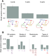
Fig 3. Topologies and properties associated with chaotic behaviour.

A Shows the models with highest posterior probability when subsetted for number of parts expressed, in order of increasing complexity (4, 5 and 6 expressed parts). The bar chart shows the mean model posterior probability across three experiments, the error bars indicate the standard deviation. B Comparison between average posterior probabilities with different properties. In order from left to right, the barcharts compare: The number of QS systems used, the modes by which QS regulates bacteriocin expression (positive, negative or both), the number of bacteriocins used, and systems containing self-limiting (SL), other-limiting (OL) or SL and OL interactions.

Fig 4. Examining chaos in m₈₅₀.

A Topology of m₈₅₀ with key parameters labelled. k_A1 is the rate of QS molecule production, KB_max1 and KB_max2 are the maximal expression rates of bacteriocins B₁ and B₂ respectively. B Posterior parameter distributions of m₈₅₀ for chaos (red) and oscillatory (blue) objectives for key parameters in system design. The borders show 1D posterior distributions for each parameter and the lower-diagonal element the 2D posterior marginals, and the upper-diagonal shows the Pearson correlations. C Feature importance calculated using random forest regression. The information gain (bits) is calculated as an average of the reduction in entropy across all trees in the forest (2000 trees). The error bars indicate the standard deviation of the entropy for each feature across all trees. D Sensitivity analysis of a chaotic input vector with chaotic region in red. Black stars refer to the identified stable steady state. The fixed parameter values are shown in Table 2

Fig 5. Parameters k_A1 and D can be tuned to control transitions between chaotic, oscillatory and stable states.

The fixed parameter values are shown in Table 2. A Map showing how different combinations of k_A1 and D change population behaviour. The grid fill colour corresponds to the maximum Lyapunov exponent measured, the grid outlines indicate the approximate classification where green is stable, yellow is oscillatory, red is chaotic and white is extinction. B Bifurcation diagram showing the community states visited for different values of k_A1. C Bifurcation diagram showing the community states visited for different values of D. D Real-time ramp down tuning of k_A1, moving the system from a chaotic state to a stable steady state. E Real-time ramp up tuning of D, moving the system from a chaotic state to a stable steady state.

Fig 6. Illustration of dual-orbit algorithm used to calculate the λ₁.

Two orbits with an initial state separation of △₀ are followed. After each time step measure the separation, △₁, is measured. The perturbed orbit (red) is readjusted to prevent excess separation. The average rate of separation between the two orbits corresponds with the λ₁.

Fig 7. Confusion matrix showing accuracy of random forest classifier on test data.

References

1. Strogatz SH. Nonlinear Dynamics and Chaos. In: Nonlinear Dynamics and Chaos; 2018.
1. Lorenz EN. Deterministic Nonperiodic Flow. Journal of the Atmospheric Sciences. 1963;20(2). doi: 10.1175/1520-0469(1963)020<0130:DNF>2.0.CO;2 - DOI
1. Ispolatov I, Madhok V, Allende S, Doebeli M. Chaos in High-Dimensional Dissipative Dynamical Systems. Scientific Reports. 2015;5. doi: 10.1038/srep12506 - DOI - PMC - PubMed
1. Albers DJ, Sprott JC, Crutchfield JP. Persistent Chaos in High Dimensions. Physical Review E—Statistical, Nonlinear, and Soft Matter Physics. 2006;74(5). - PubMed
1. Dechert WD, Sprott JC, Albers DJ. On the Probability of Chaos in Large Dynamical Systems: A Monte Carlo Study. Journal of Economic Dynamics and Control. 1999;23(8). doi: 10.1016/S0165-1889(98)00053-0 - DOI
Publication types