Flexible neural control of motor units

Abstract

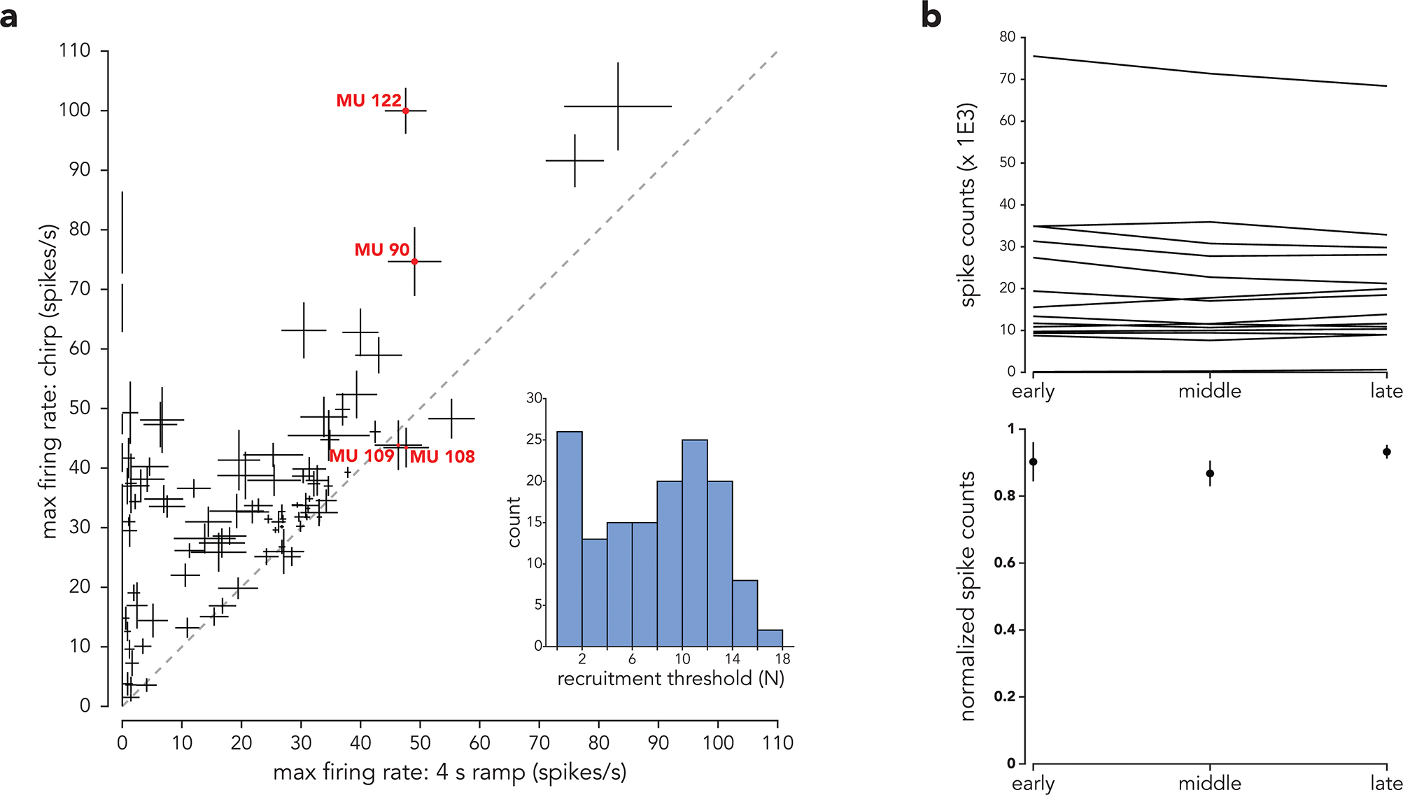
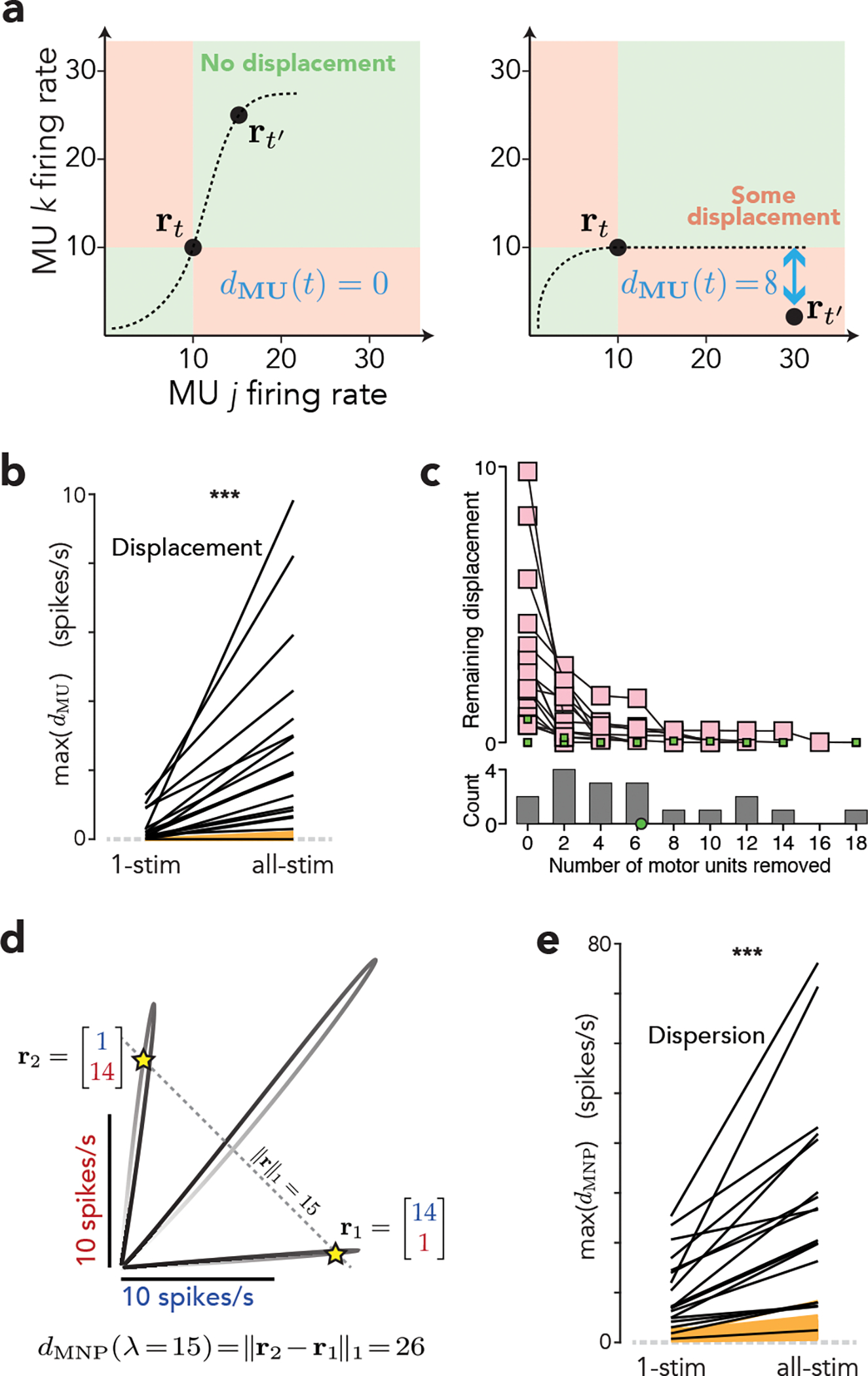
Voluntary movement requires communication from cortex to the spinal cord, where a dedicated pool of motor units (MUs) activates each muscle. The canonical description of MU function rests upon two foundational tenets. First, cortex cannot control MUs independently but supplies each pool with a common drive. Second, MUs are recruited in a rigid fashion that largely accords with Henneman's size principle. Although this paradigm has considerable empirical support, a direct test requires simultaneous observations of many MUs across diverse force profiles. In this study, we developed an isometric task that allowed stable MU recordings, in a rhesus macaque, even during rapidly changing forces. Patterns of MU activity were surprisingly behavior-dependent and could be accurately described only by assuming multiple drives. Consistent with flexible descending control, microstimulation of neighboring cortical sites recruited different MUs. Furthermore, the cortical population response displayed sufficient degrees of freedom to potentially exert fine-grained control. Thus, MU activity is flexibly controlled to meet task demands, and cortex may contribute to this ability.

Extended Data Fig. 1. Example MU spikes and sorting, including a challenging moment with spike overlap.

Behavior and MU responses during one dynamic-experiment trial. The target force profile was a chirp. Top: generated force. Middle: eight-channel EMG signals recorded from the lateral triceps. 20 MUs were isolated across the full session; 13 MUs were active during the displayed trial. MU spike times are plotted as circles (one row and color per MU) below the force trace. EMG traces are colored by the inferred contribution from each MU (since spikes could overlap, more than one MU could contribute at a time). Bottom left: waveform template for each MU (columns) and channel (rows). Templates are 5 ms long. As shown on an expanded scale (bottom right), EMG signals were decomposed into superpositions of individual-MU waveform templates. The use of multiple channels was critical to sorting during challenging moments such as the one illustrated in the expanded scale. For example, MU2, MU5, and MU10 had very different across-channel profiles. This allowed them to be identified when, near the end of the record, their spikes coincided just before the final spike of MU12. The ability to decompose voltages into a sum of waveforms also allowed sorting of two spikes that overlapped on the same channel (e.g., when the first spike of MU6 overlaps with that of MU10, or when the first spike of MU9 overlaps with that of MU5). The fact that sorting focused on waveform shape across time and channels (rather than primarily on amplitude) guarded against mistakenly sorting one unit as two if the waveform scaled modestly across repeated spikes (as occurred for a modest subset of MUs).

Extended Data Fig. 2. Basic properties of MU responses.

(a) Comparison, for all MUs recorded during the dynamic experiments, of maximum rates during the four-second increasing ramp and during the chirp. Each point plots the maximum trial-averaged firing rate and its standard error for one MU (N = number of trials for that MU and that condition; 28 on average). Labels highlight four MUs that have similar maximum firing rates during the ramp but different maximum firing rates during the chirp. There were also many MUs that were nearly silent during the ramp but achieved high rates during the chirp (points clustered near the vertical axis). Inset: distribution of recruitment thresholds, estimated as the force at which the MU’s firing rate, during the four-second ramp condition, exceeded 10% of its maximum rate during that condition. (b) Analysis of the possible impact of fatigue across the course of each session. Top: total MU spike counts, over the full recorded population, after dividing the session into thirds. Each line corresponds to one session. Bottom: Mean and standard error (across 14 sessions) of the normalized total MU spike counts (counts for each session were normalized by maximum across trial epochs). There is little overall change in MU activity over the course of a session.

Extended Data Fig. 3. Additional documentation of single-trial responses during a dynamic experiment session.

Presentation is similar to Fig. 5a–c but voltage traces are shown for six total trials. Furthermore, spike rasters are shown for all active MUs and all trials for two conditions: the four-second ramp and the 3 Hz sinusoid. (a) Same as Fig. 5a but force traces are highlighted for six trials (three trials per condition) rather than two. (b) MU spike templates, repeated from Fig. 5b. (c) EMG voltage traces for the highlighted trials and times (slightly greater time ranges are used relative to Fig. 5c). Data are shown for six trials, three in each column. Four recording channels are shown per trial. Left column: three trials for the ramp. Right column: three trials for the sinusoid. In each column, the second trial repeats that shown in Fig. 5c. Vertical and horizontal scales are shared with panel b. (d) Responses of all MUs that were active for these two conditions during this session. Data is shown for the four-second ramp (left column) and the 3 Hz sinusoid (right column). Data is color-coded by MU. Labels give both the session-specific MU identity (1–7), and the overall ID. Trial-averaged rates are shown with flanking standard errors. Spike rasters contain one row per trial, ordered from the first trial for that condition at the bottom to the last at top. Trials for all conditions were interleaved during the experiment. Vertical scale: 20 spikes/s. Horizontal scale: 500 ms.

Extended Data Fig. 4. Example MU responses and waveforms across muscle lengths.

These data address a potential artifact: an apparent change in recruitment across muscle lengths could occur if, due to tiny shifts in electrode location across muscle lengths, the spikes of an MU become undetectable. On the one hand, the stability of neighboring MUs largely rules out this concern. On the other hand, it is conceivable that most MUs could remain stable, while one (or more) MUs undergo a dramatic change in waveform that renders them unsortable. Addressing this concern thus requires confirming that changes in recruitment are observed concurrently with waveform stability. (a) State-space plots illustrating, for two MUs, that changes in muscle length create large departures from a 1D monotonic manifold. Departures occurred because the activity of MU158 was greatly reduced when muscle length was shortened. A natural concern is thus that the waveform of MU158 may have changed (or disappeared) across muscle lengths, causing an apparent drop in firing rate due to most spikes being missed. If one considered only the data for the 2 Hz sinusoid, this potential confound cannot be ruled out because there are no spikes from MU158 during that condition. Thus, one cannot distinguish between the possibility that MU158 is no longer detectable and the possibility that it is no longer active. However, other conditions did evoke activity from MU158. Thus, MU158 is still detectable, it is just much less active. (b) The above observations largely rule out the concern that the drop in firing rate of MU158, at the shorter muscle length, is due to it becoming undetectable. Yet perhaps its waveform changed considerably – enough to be detected only occasionally? Alternatively, perhaps MU158 did indeed become undetectable, and the spikes attributed to it were from some other MU? Both these possibilities are very unlikely: waveform shape, across multiple channels, provided a unique signature of this MU that was stable across muscle lengths. Left. Template of MU158 across the 5 EMG channels used during this session. Middle. Across all conditions when the muscle was long, we sorted 5147 spikes matching the template. The 20 with the best match are shown. Right. Across all conditions when the muscle was short, we sorted 1568 spikes that matched the template (~30% as many spikes as when the muscle was long). The 20 with the best match are shown, and illustrate that this waveform was still very much present. This rules out the concern that the waveform of MU158 has changed dramatically. It also addresses the concern that the waveform of MU158 has become undetectable, and the apparent spikes of MU158 are due to missorted spikes from some other MU. This is extremely unlikely; the ‘other’ MU would have to produce spikes that matched the original template, across both time and channels.

Extended Data Fig. 5. Single-latent model fits to artificial data constructed to be consistent with rigid control, but with various types of noise.

We generated realistic simulated data from a 1-latent model by fitting our 1-latent model to the empirical MU response from one session. Then, using the learned latents, link functions, and lags, we generated simulated MU activity. We then fit a different model (with different initialization or parameters) to confirm that it could successfully fit the simulated responses. This acts as both a test of whether optimization succeeds in finding a perfect fit when one is possible, and as a way of documenting the behavior of the cross-validated fit error. (a) ‘True’ (gray traces) and model fit (dashed red traces) responses for two example simulated MUs (columns) during four conditions (rows). Simulations involved no sampling error. R² values of the fit were above 0.99 for all MUs. (b) Cross-validated error plots (as in Fig. 7) for simulated data for this example session, and after incorporating noise into the simulations. ‘Independent emission noise’ is Gaussian noise that is independently added at each time point, with standard deviation for each MU equal to the SEM of MU activity across trials (a typical value was found by averaging across time-points and MUs). ‘Realistic emission noise’ is T-dimensional gaussian noise (where T is the number of time points) generated from a MU's temporal covariance structure computed across trials (i.e., the covariance matrix of a T × R matrix of activity, where R is the number of trials). This noise structure is calculated separately for each MU. ‘Realistic latent noise’ is T-dimensional gaussian noise that is added to the latent (prior to the link functions), rather than noise directly added to the MU activities. This noise was generated from the latents' temporal covariance structure computed across trials. Independent noise was added to the latent for each MU, corresponding to each neuron receiving a noisy version of a single latent. Error bars show mean and 95% range of the cross-validation error across 10 partitionings of the data. Note that cross-validated error should be zero on average if sampling noise is the only impediment to a perfect fit, and is thus expected (in that situation) to take on a range of positive and negative values centered near zero. Cross-validated error was indeed near zero for all simulations (and much lower than the fit error for the empirical data, orange) confirming that optimization was successful and cross-validated error behaved as expected. Note that this session had larger single-latent model violations for the empirical data than the average session, so the scale of the y-axis is larger than in Fig. 7.

Extended Data Fig. 6. Example M1 neural activity.

(a) Trial-averaged forces from one recording session. Each column corresponds to one condition (the intermediate static force condition is omitted for space). Vertical scale bar indicates 8 N. Horizontal scale bar indicates 1 s. (b-j) Responses of 9 M1 neurons. Each subpanel plots the trial-averaged firing rate with standard error (top) and single-trial spike rasters (bottom). Vertical scale bars indicate 20 spikes/s. Horizontal scale bars indicate 1 s.

Figure 1 |. Rigid versus flexible motor unit control and experimental setup.

(a) Rigid control schematic. The activity of many MUs is determined by a small number of force commands. Commands may be for individual-muscle force, or may be ‘synergies’ that control a mechanical action (e.g., an elbow flexion synergy and a forearm supination synergy). Thus, the number of controlled degrees of freedom is less than or equal to the number of motor neuron pools. Each MU’s activity is a ‘link function’ of one synergy (or for multifunctional muscles, 2–3 synergies). Link functions typically enforce size-based recruitment. (b) Flexible control schematic. Each motor neuron pool is controlled by multiple degrees of freedom, such that recruitment can be size-based but can also be flexibly altered when other solutions are preferable. (c) Task schematic. A monkey modulated the force generated against a load cell to control Pac-Man’s vertical position and intercept a scrolling dot path. (d) Single-trial (gray), trial-averaged (black), and target (cyan) forces from one session. Vertical scale: 4 N. Horizontal scale: 500 ms.

Figure 2 |. Stimulation experiments.

(a) Microstimulation was delivered, on interleaved trials, through a selection of electrodes on a linear array. (b) EMG voltages for two EMG recording channels (of eight total) and four example trials, stimulating on electrode 23 or 27. The two electrodes recruited MUs with different waveform magnitudes, and vertical scales are adjusted accordingly. Stimulation was delivered during each green-shaded region, during which a small stimulation artifact can be seen. Right. spike templates for these two MUs. Vertical scale: 50 standard deviations of background noise (ignoring stimulation artifact). (c) Responses of the same two MUs, for all trials during stimulation on three electrodes. Traces plot firing rates (mean and standard error). Rasters show spike times, separately for the two MUs. (d) As in c but for a different session. (e) Additional example from a different session, showing responses during both the four-second ramp and during stimulation as the monkey held two baseline force levels. Mean force plotted at top. (f) As in e, but for a different session. (g) State-space predictions for rigid control (left) and flexible control (right). (h) State-space plots for two sessions where MUs were recorded from the lateral deltoid. Each subpanel plots joint activity of two MUs during stimulation on each of three electrodes. (i) For two sessions recording from sternal pectoralis major. Left: activity during stimulation on three electrodes. Right: activity during stimulation on two electrodes and during the slow force ramp. (j), For two sessions recording from lateral triceps.

Figure 3 |. Quantifications of flexible control.

(a) Schematic illustrating MU displacement (d_MU) for a two-dimensional population state and two times. Left. a monotonic manifold can pass through r_t and ${\mathbf{r}}_{t^{\prime }}$. Thus, d_MU(t) = 0. Right. Any monotonic manifold passing through r_t is restricted to the green zone, and thus cannot come closer than 8 spike/s to ${\mathbf{r}}_{t^{\prime }}$. Thus, d_MU(t) = 8. (b) Maximum displacement (one black line per session). For ‘1-stim’, displacement was computed across times during the response for each stimulation site alone. The maximum was then taken across sites from that session. For ‘all-stim’, the maximum displacement was computed across all times and stimulation sites within a session. ‘All-stim’ displacement was significantly larger (two-sample two-tailed t-test, p = 0.00017, N=18 sessions). Both were significantly larger than the displacement expected due to sampling error alone (yellow, ten resampled artificial populations per empirical dataset). (c) Maximum displacement (for ‘all-stim’) after repeatedly removing the MU pair causing the largest displacement. Each trace corresponds to one session, and ends when remaining displacement is no larger than the largest across the ten resampled populations for that session. Gray histogram plots the distribution, across sessions, of the number of MUs that had to be removed to reach that point (mean in green). (d) Illustration of MNP dispersion metric for two MUs. The three trajectories were driven by stimulation at three cortical sites. The line defined by ∥r∥₁ = 15 intercepts these trajectories at six points, with r₁ and r₂ being most distant. The MNP dispersion for λ = 15 is the L1 distance between these points. (e) Maximum (across λ) dispersion (one line per session). ‘All-stim’ dispersion was significantly larger (two-sample two-tailed t-test, p = 0.00011, N=18 sessions). Both were significantly larger than the dispersion expected due to sampling error alone (yellow, ten resampled artificial populations per empirical dataset). Results are shown for conditions where stimulation was delivered as the monkey held a low static force, and were nearly identical for a higher static force.

Figure 4 |. Optimal MU recruitment.

(a) Isometric force production was modeled using an idealized MNP containing 5 MUs. MU twitch amplitude varied inversely with contraction time such that small MUs were also slow. A given set of rates resulted in both a mean total force and inferred trial-to-trial variation around that force. The latter was smaller when using multiple small MUs versus one large MU. Both contributed to mean-squared error between actual and target forces. The optimal set of MU firing rates was numerically derived as the solution minimizing that error. Optimization was independent for each force profile. (b) Example target (cyan) and mean MNP (black) forces (for simplicity no variability is shown). Mean force matched targets very well, with notable small exceptions at the troughs during sinusoidal forces. (c) Optimal MU firing rates, used to generate the forces in b. Each color corresponds to a different MU, numbered by size (MU1 was the smallest and slowest). (d) State space plot of MU3 versus MU2 for each condition in c.

Figure 5 |. Dynamic experiments.

(a) Forces for two conditions: the four-second ramp and the 3 Hz sinusoid. Gray traces show all trials in this session. Black traces highlight trials for which EMG data are shown below. (b) MU spike templates across four (of eight) EMG channels recorded in the lateral triceps. Vertical scale: 50 standard deviations of the noise. Each template spans 10 ms. (c) EMG voltage traces for the two trials and time-periods highlighted in a. Traces become colored to indicate when spikes were detected. Numbers indicate the identity of the MU producing the spike. In some cases, spikes from two or more MUs overlap. Trace color reflects the relative magnitudes of the contributions made by different MUs. (d) Responses of two MUs during the 0.25 Hz sinusoid. Black trace at top shows trial-averaged force. Colored traces show firing rates (mean and standard error). Rasters show individual spikes on all trials for these conditions. Vertical scales: 8N and 20 spikes/s. (e) Response of two MUs during the four-second ramp (left) and 3 Hz sinusoid (right). MU311 and MU309 correspond to MUs 3 and 5 for the session focused on in c. (f) Response of two MUs (from a different session) during the four-second ramp (left) and the 0 – 3 Hz chirp (right). (g) Response of two MUs (from a different session) during the 250 ms increasing and decreasing ramps. (h,i,j) State-space plots for the MUs shown in d,e,f. Scale bars: 20 spikes/s. (k) Maximum displacement for every session. Displacement was computed twice: within the four-second ramp only, and again across all conditions. Yellow lines plot displacement expected due to sampling error (ten resampled artificial populations per session). Empirical slopes were significantly larger than expected given sampling error (two-sample two-tailed t-test, p = 0.000003, N=14 sessions). (l) Maximum displacement, across all conditions, after repeatedly removing the MU pair that caused the largest displacement. Each trace corresponds to one session, and ends when remaining displacement was no larger than the largest from the ten resampled datasets (or when no pairs would be left). Gray histogram plots the distribution, across sessions, of the number of MUs that had to be removed (mean in green). One session (lone green square) terminated immediately because it contained only 3 MUs. (m) Cumulative distribution for displacement (d_MU(t)). Rather than summarizing a session by taking the maximum across all times (as in k,l), here we plot the distribution of d_MU(t) for all times within one session. Distributions were computed for the slowly increasing ramp alone (purple) and all conditions (green). (n) Maximum (across λ) dispersion (one line per session). Slopes were significantly larger than expected given sampling error (two-sample two-tailed t-test, p = 0.0000007, N=14 sessions). (o) Additional within-session analysis of dispersion. Rather than summarizing a session by taking the maximum d_MNP(λ) across λ (as in n), here we plot d_MNP(λ) versus the λ (the norm).

Figure 6 |. Muscle-length experiments.

The monkey generated a subset of the force profiles in Fig. 1d with a shoulder-flexion angle of 15° (the deltoid was long) or 50° (the deltoid was short). (a) Example forces and recordings when the deltoid was long, for one static-force condition. Gray traces plot force for all trials. Black trace plots force for one example trial. EMG voltages traces are shown for the highlighted portion (gray window) of that trial. Only two channels are shown for simplicity. Conventions as in Fig 5c. (b) Same but for later in the session after posture was changed and the deltoid was short. Recordings are from the same two channels and many of the same MUs (MU1, MU3, and MU4) are visible. However, MU4 has become considerably less active and MU5 is now quite active, despite being rarely active when the deltoid was long. (c) Data, from the same session documented in a,b, recorded during the 250 ms decreasing ramp. MU158 and MU159 correspond to MU4 and MU5 from panels a,b. Gray traces at top plot trial-averaged force. Colored traces plot firing rates (mean and standard errors). Rasters show spikes on all trials for this condition. Top and bottom subpanels plot data where the deltoid was long and short. (d) Example from another session, recorded during the 0 – 3 Hz chirp. (e) State space plots for four example MU pairs. Top-left: same data as in c. Bottom-left: same data as in d. Top-right: additional comparison from the same session documented in a,b. MUs 157 and 158 correspond to MUs 3 and 4. Responses are during the chirp. Bottom-right: Example from a different session. Responses are during the 250 ms downward ramp. (f) Maximum displacement for every session (one line per session). Displacement was computed three times: within the four-second ramp, across all conditions within a muscle length (then pooled across lengths), and across all conditions and both muscle lengths. Yellow lines plot displacement expected due to sampling error (ten resampled artificial populations per empirical dataset). The empirical slopes were significantly larger than expected due to sampling error both for the increase from the four-second ramp to all conditions within a muscle length (p = 0.00044) and for the additional increase when considering both muscle lengths (p = 0.022, two-sample two-tailed t-test, N=6 sessions). (g) Maximum displacement (across all conditions and both muscle lengths) after repeatedly removing the MU pair that caused the largest displacement. Each trace corresponds to one session, and ends when remaining displacement was no larger than the largest within the ten resampled populations. Gray histogram plots the distribution, across sessions, of the number of MUs that had to be removed (mean in green). (h) Cumulative distribution of displacement, within one session, for the three key comparisons: four-second ramp (purple), all conditions within a muscle length (green), and all conditions for both muscle lengths (orange), for one session. (i) As in f but for dispersion. The two slopes were significantly higher than expected given sampling error (p = 0.00011 and p = 0.03, two-sample two-tailed t-tests, N=6 sessions). (j) d_MNP(λ) as a function of the norm, λ, for one session.

Figure 7 |. Latent factor model.

(a) The model embodies the premise of rigid control: MU firing rates are fixed ‘link functions’ of a shared, 1-D latent input. (b) Model performance for the three experiment types. The model was fit separately for each session. Regardless of how many conditions were fit, error was computed only during the four-second ramp. To compute cross-validated error, each session’s data was divided, trial-wise, into two random partitions. The model was fit separately to the mean rates for each partition. For each MU, cross-validated fit error was the dot product of the two residuals. To summarize cross-validated error for that experiment type, we computed the median error across all MUs in all relevant sessions. Partitioning was repeated 10 times. Vertical bars indicate the mean and standard deviation across these 10 partitionings, and thus indicate reliability with respect to sampling error (the standard deviation of the sampling error is equivalent to the standard error). Purple bars plot error when fitting only the four-second ramp. Green bars plot error when fitting additional conditions (stimulation across multiple sites, or different force profiles). For muscle-length experiments, green bars plot error when fitting all force profiles for the same muscle length, then averaging across muscle lengths. Orange bars plot error when fitting all force profiles for both muscle lengths. Circles show cross-validated fit error for an artificial population response that obeyed rigid control, but otherwise closely resembled the empirical population response. (c) Illustration of model fits for simplified situations: the activity of two MUs during the four-second ramp (top) or following cortical stimulation on three different electrodes (bottom). For illustration, the model was fit only to the data shown. (d) Proportion of total MUs that consistently violated the single-latent model when fit to pairs of conditions. Each entry is the difference between the proportion of consistent violators obtained from the data and the proportion expected by chance. Left: dynamic experiments. Right: for muscle length experiments, we grouped conditions by frequency (lower on top, higher on bottom).

Figure 8 |. Quantifying neural degrees of freedom.

(a) Schematic illustrating the central question: how many degrees of freedom might influence the MNP? (b) Cross-validated fit error as a function of the number of latent factors. Cross-validated error was computed within all conditions, but was otherwise calculated as above. For each partitioning, the overall error was the median cross-validated error across all MUs in two sessions. Error bars indicate the mean +/− standard deviation across 10 total partitionings. (c) We recorded neural activity in motor cortex using 128-channel Neuropixels probes. (d) Two sets of trial-averaged rates were created from a random partitioning of trials. Traces show the projection of the first (green) and second (purple) partitions onto PCs found using only the first. Traces for PCs 1 and 50 were manually offset to aid visual comparison. (e) Reliability of neural latent factors for the first 60 factors. Traces plot the mean and central 95% (shading) of the distribution across 25 random partitionings. (f) Same but for latent factors 1–400. The empirical reliability (blue) is compared to that for simulated data with 50 (yellow), 150 (orange), and 500 (red) latent signals.

References

1. Enoka RM & Pearson KG The motor unit and muscle action. in Principles of Neural Science 768–789 (2013).
1. Burke RE et al. An HRP study of the relation between cell size and motor unit type in cat ankle extensor motoneurons. J Comp Neurol 209, 17–28 (1982). - PubMed
1. Buchthal F & Schmalbruch H Contraction times and fibre types in intact human muscle. Acta Physiol Scand 79, 435–452 (1970). - PubMed
1. Gokhin DS et al. Thin-filament length correlates with fiber type in human skeletal muscle. Am J Physiol-cell Ph 302, C555–C565 (2012). - PMC - PubMed
1. Nardone A, Romanò C & Schieppati M Selective recruitment of high-threshold human motor units during voluntary isotonic lengthening of active muscles. J Physiology 409, 451–471 (1989). - PMC - PubMed
Methods-only References
1. Stephens JA, Garnett R & Buller NP Reversal of recruitment order of single motor units produced by cutaneous stimulation during voluntary muscle contraction in man. Nature 272, 362–364 (1978). - PubMed
1. Graziano MSA, Taylor CSR & Moore T Complex Movements Evoked by Microstimulation of Precentral Cortex. Neuron 34, 841–851 (2002). - PubMed
1. Loeb GE & Gans C Electromyography for Experimentalists. (The University of Chicago Press, 1986). doi: 10.2307/1445582. - DOI
1. Steinmetz NA et al. Neuropixels 2.0: A miniaturized high-density probe for stable, long-term brain recordings. Biorxiv 2020.10.27.358291 (2020) doi: 10.1101/2020.10.27.358291. - DOI - PMC - PubMed
1. Quiroga RQ, Nadasdy Z & Ben-Shaul Y Unsupervised spike detection and sorting with wavelets and superparamagnetic clustering. Neural Comput 16, 1661–1687 (2004). - PubMed
Publication types