Fast and scalable search of whole-slide images via self-supervised deep learning

Abstract

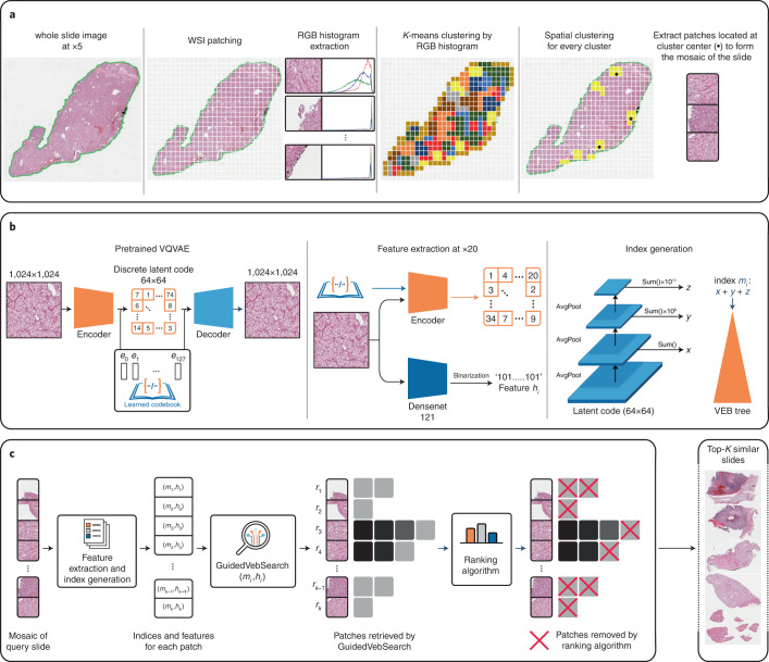
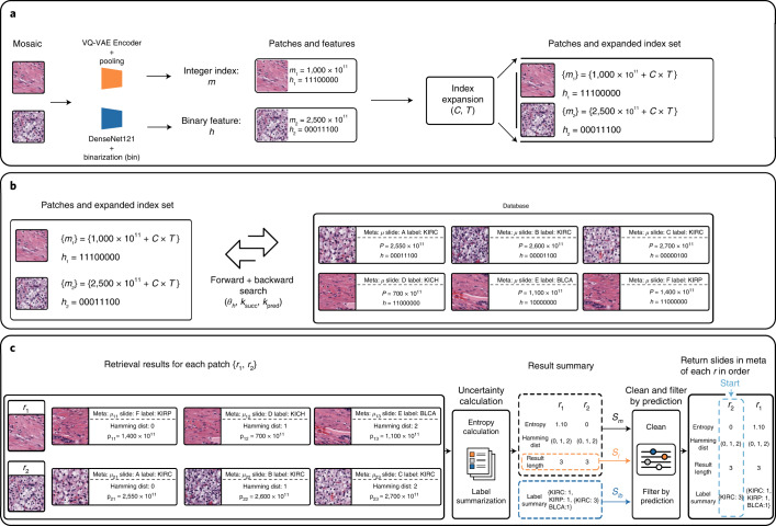
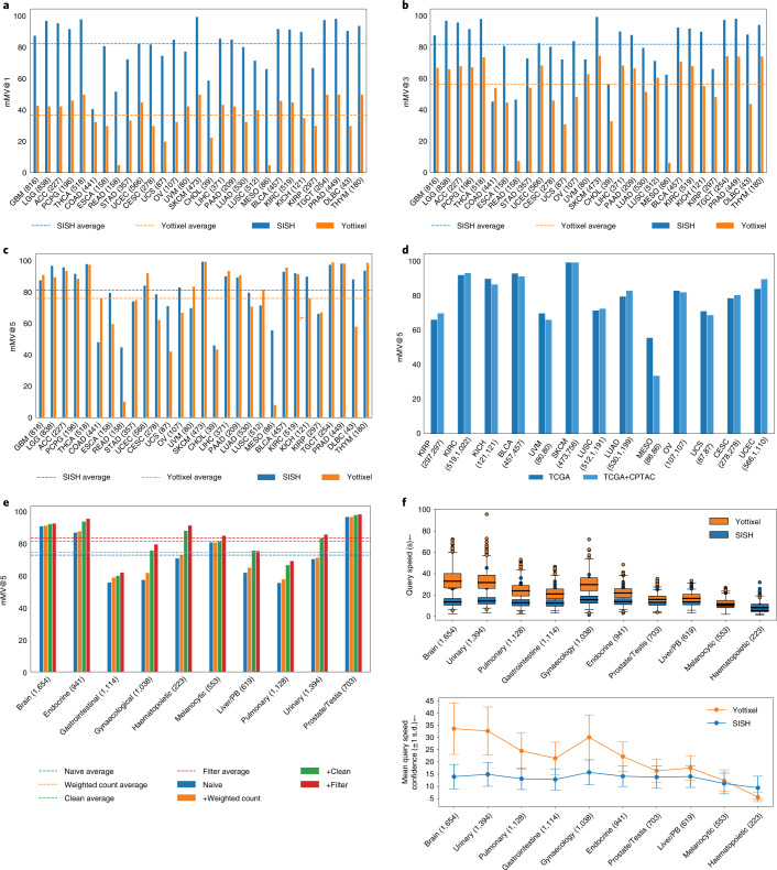
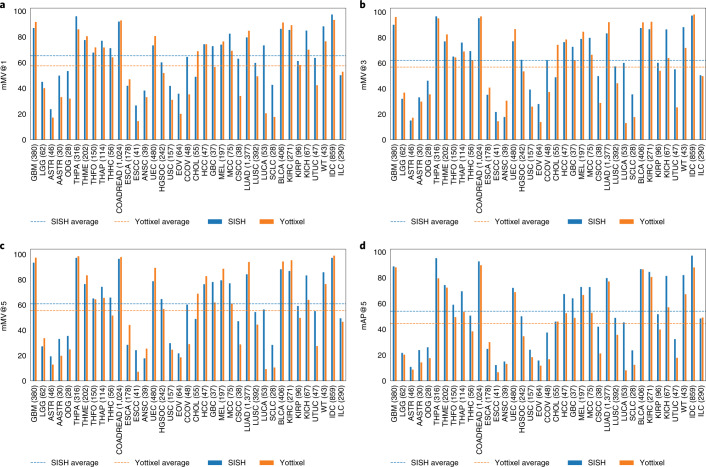
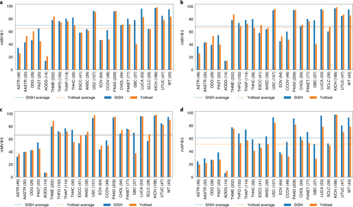
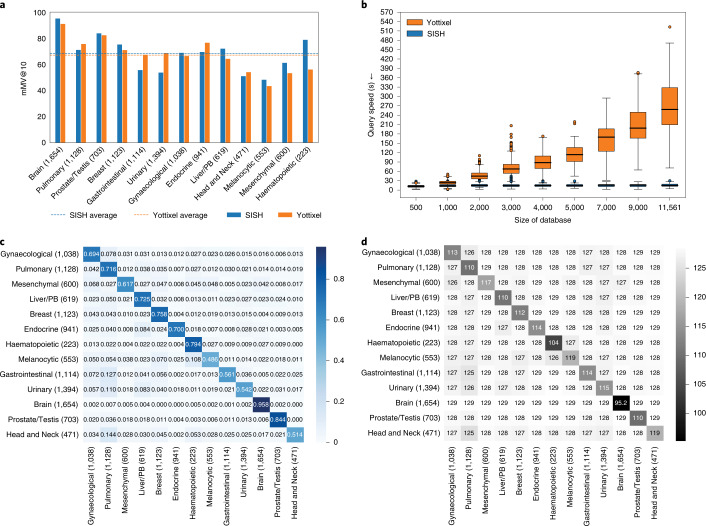
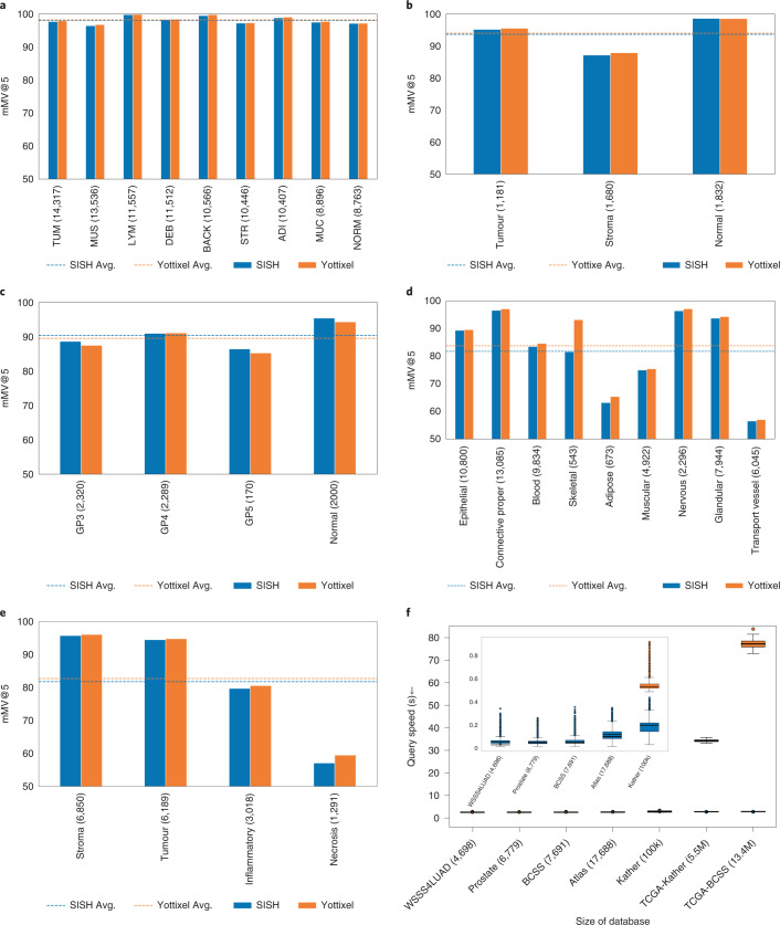
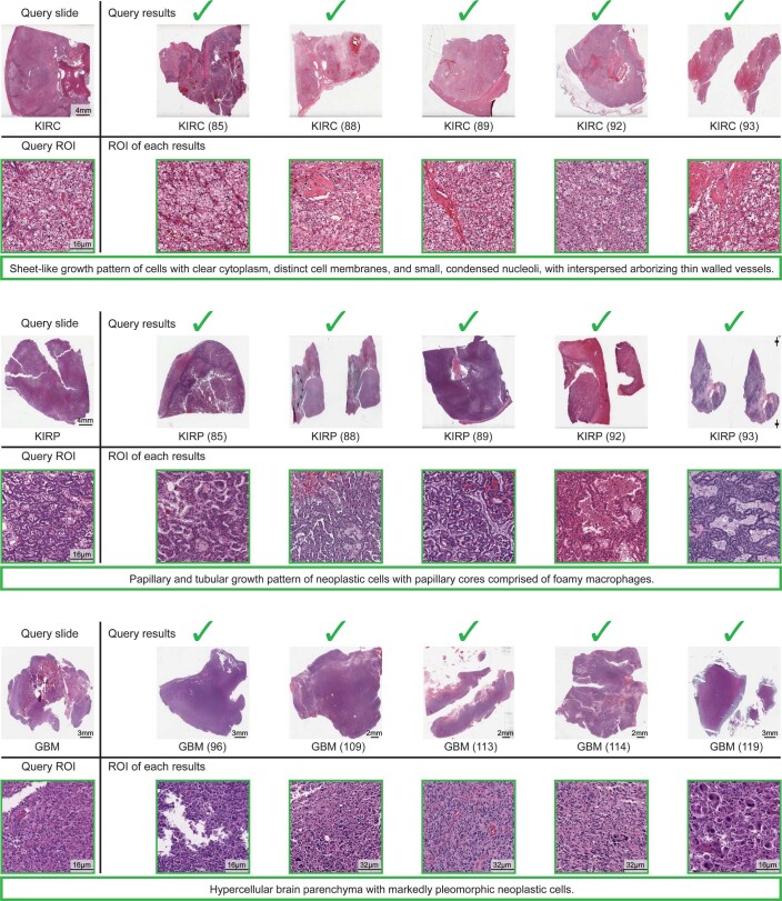
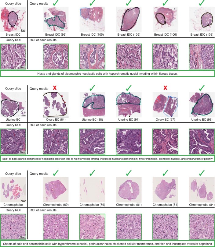
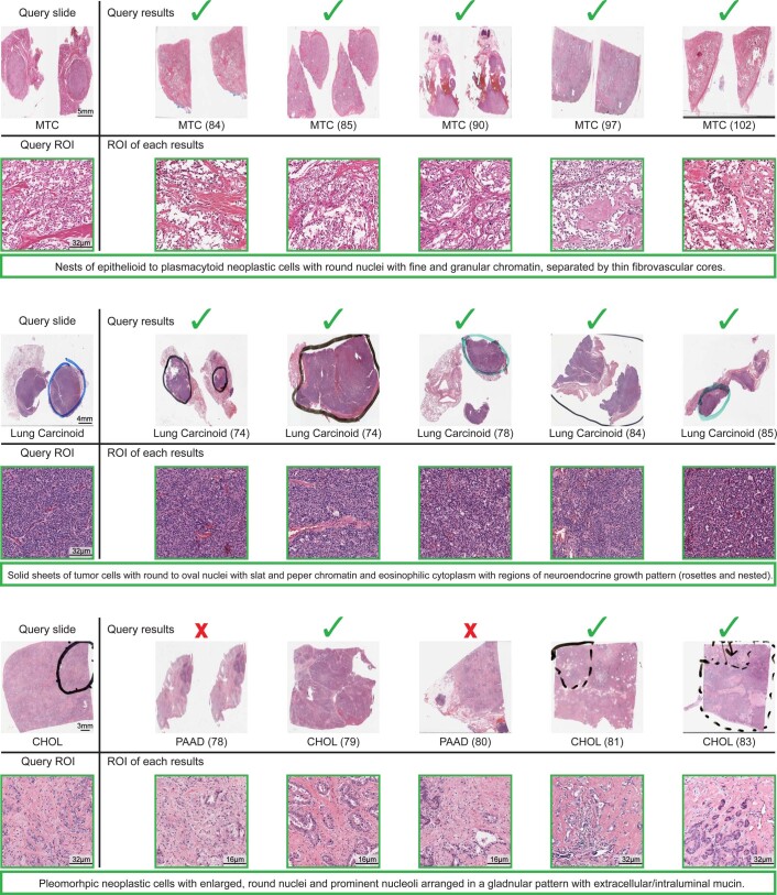
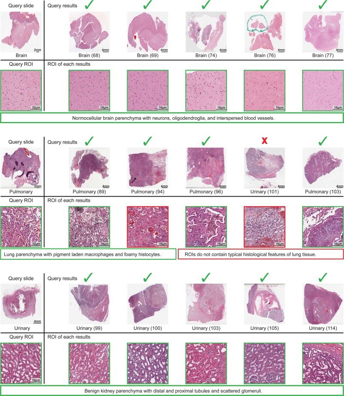
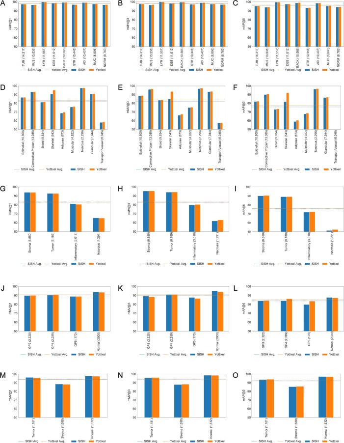
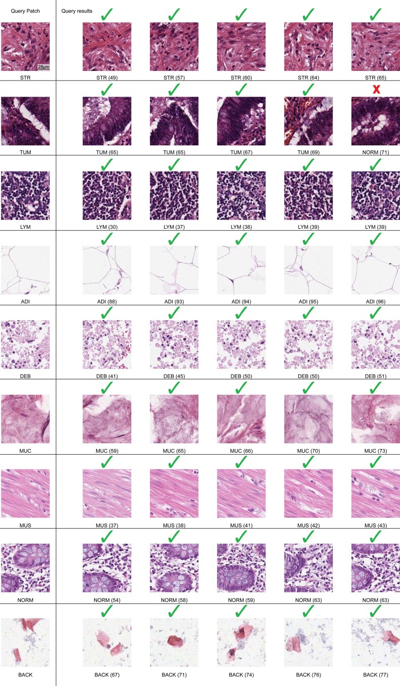
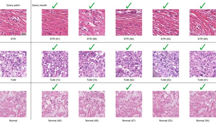
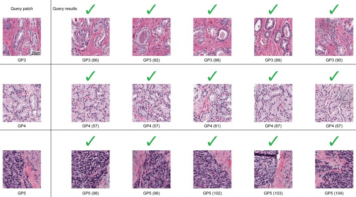
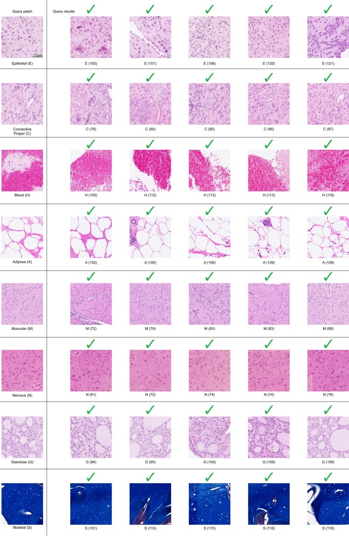
The adoption of digital pathology has enabled the curation of large repositories of gigapixel whole-slide images (WSIs). Computationally identifying WSIs with similar morphologic features within large repositories without requiring supervised training can have significant applications. However, the retrieval speeds of algorithms for searching similar WSIs often scale with the repository size, which limits their clinical and research potential. Here we show that self-supervised deep learning can be leveraged to search for and retrieve WSIs at speeds that are independent of repository size. The algorithm, which we named SISH (for self-supervised image search for histology) and provide as an open-source package, requires only slide-level annotations for training, encodes WSIs into meaningful discrete latent representations and leverages a tree data structure for fast searching followed by an uncertainty-based ranking algorithm for WSI retrieval. We evaluated SISH on multiple tasks (including retrieval tasks based on tissue-patch queries) and on datasets spanning over 22,000 patient cases and 56 disease subtypes. SISH can also be used to aid the diagnosis of rare cancer types for which the number of available WSIs is often insufficient to train supervised deep-learning models.

Fig. 1. Overview of the SISH pipeline.

a, After tissue segmentation, we tile the foreground regions and perform two-stage K-means clustering to select representative patches to include in the WSI mosaic. We first cluster all patches based on their RGB histogram features. In each cluster generated from the first stage (for example, the yellow cluster shown in the figure), we perform K-means clustering again using the spatial coordinates of each patch as features (spatial clustering), extract the patches that correspond to the coordinates of each resulting cluster centre (black dots) and add them to the mosaic of the slide. b, We pretrain a VQ-VAE on tissue patches from slides in the TCGA and save its encoder and codebook for feature extraction. For each patch in the mosaic, the VQ-VAE encoder is used to compute its discrete latent representation and a Densenet121 encoder is used to obtain a binarized texture feature vector. Finally, we feed the discrete latent representation into another pipeline composed of a series of average pooling (AvgPool), shift and summation operations to get an integer index for the patch, then use the vEB tree to construct the index structure for search. c, For a given query slide preprocessed as a mosaic representation, we feed the mosaic into the feature extractor to compute the integer indices and binarized texture features of each patch in the mosaic, then apply our search and ranking algorithm to filter the candidate patches. See Fig. 2 for more details.

Fig. 2. Detailed illustration of search.

a, Starting from the mosaic of a WSI where a patch could contain normal tissue or morphology of a cancer subtype, SISH encodes each patch into both an integer and binary string representation, using a VQ-VAE encoder and a DenseNet121 encoder pretrained on ImageNet respectively. The pooling operation consists of a series of average pool, summation and multiplication explained in Methods. The binarization process converts a continuous vector to a binary string by starting from ∞, then walking through all elements in the vector to compare the value of the current element to that of the next one. If the next value is smaller than the current, it assigns the current value to 0, and 1 otherwise. Afterwards, for each patch in the mosaic, SISH expands its index into a set of candidate indices. C and T are hyperparameters used during expansion (see Guided search algorithm section of Methods). b, For each patch, SISH applies the search function to each index in the set of candidate indices. The search function returns the patches within k_succ successors and k_pred predecessors in the database whose Hamming distance from the patch in the query mosaic is smaller than θ_h. Each patch in the database is associated with an index p and metadata μ defined in Methods. c, For each result r, SISH calculates its entropy (by considering the frequency of occurrence of slide labels) and returns summary variables S_m, S_l and S_lb for cleaning. In the example shown in the figure, the cleaning function removes outliers in {r₁, r₂}. A result r is considered as an outlier if its length (number of patches retrieved) is greater than the O_h or smaller than the O_l percentile. At the same time, the function also removes patches within each r whose Hamming distance is greater than the average of the top-k in r. Lastly, SISH takes a majority vote of the top-5 slide labels within each r to remove patches whose slide labels disagree with the majority vote and extract the slides from the r with the lowest entropy (see the corresponding sections in Methods for details of entropy calculation, clean and filter-by-prediction).

Fig. 3. Disease subtype retrieval in public cohorts.

a–c, Macro-average mMV@1,3 and 5 of SISH and Yottixel on the TCGA anatomic sites. SISH has better performance in all metrics, especially mMV@1 and mMV@3. d, Comparison between SISH on TCGA and TCGA+CPTAC cohorts. The performance does not vary before and after mixing with CPTAC cohorts for most cases. e, Ablation study result for the ranking module of SISH. We observed that SISH achieves best performance in the setting where all functions are applied (+filter) (details of each setting are described in Methods (Ablation study). f, Top: query speed comparison between SISH and Yottixel for each site. The box extends from the first quartile (Q1) to the third quartile (Q3) of the data and the whiskers extend from the box by 1.5× the interquartile range (IQR). Bottom: the mean confidence (±1 s.d.) of query speed between SISH and Yottixel. It is crucial to note that SISH is 2× more effective when the number of slides is over 1,000 (details on the study of speed is reported in Speed and interpretability. Numbers in parentheses denote the number of WSIs for all panels except d, where numbers in parentheses denote the number of WSIs in TCGA and TCGA+CPTAC, respectively. Source data

Fig. 4. Adapting to the BWH independent test cohort.

a–c, Average mMV@1, 3 and 5 scores of SISH and Yottixel for each subtype in BWH general cohorts. SISH achieved higher scores than Yottixel by 7.87%, 5.33% and 5.33% for mMV@1, 3 and 5, respectively. d, mAP@5 score of SISH and Yottixel. SISH outperformed Yottixel in 34 out of 37 subtypes, resulting in 9.5% higher mAP@5 score. Numbers in parentheses denote the number of WSIs. Source data

Fig. 5. Adapting to rare cancer types.

a–c, Macro-average mMV@1, 3 and 5 scores of SISH and Yottixel in each rare cancer subtype. SISH achieved higher mMV1 and 3 scores than Yottixel by 4.56% and 2.42%, respectively. d, Macro-average mAP@5 score. SISH outperformed Yottixel in 22 out of 23 subtypes by 9.82%. Numbers in parentheses denote the number of WSIs. Source data

Fig. 6. Performance on anatomic site retrieval and speed.

a, mMV@10 comparison between SISH and Yottixel. b, Speed comparison between SISH and Yottixel in the TCGA anatomic site retrieval. SISH is faster than Yottixel by approximately 15× when the number of slides is over 10,000. See Speed and interpretability for more details. The box extends from Q1 to Q3 of the data and the whiskers extend from the box by 1.5 × IQR. c,d, Confusion matrix (c) and Hamming distance matrix (d) of SISH for anatomic site retrieval. The x and y axes correspond to the model prediction and ground truth, respectively. The sharp diagonal line in both matrices show that SISH can retrieve the correct results and avoid the dissimilar ones in most cases. Numbers in parentheses denote the number of WSIs from each site. PB, pancreaticobiliary. Source data

Fig. 7. Patch-level retrieval.

a–e, mMV@5 results for SISH and Yottixel for patch level retrieval on multiple patch level datasets: Kather100k, WSSS4LUAD, BWH prostate, Atlas and BCSS datasets. SISH performed similarly to Yottixel on all datasets. f, Query speeds of SISH and Yottixel. SISH achieved faster mean query speed by a factor of 3 to 230 as the size of the database grew from 100,000 to 13.4 million images. The results were averaged across query times of all data in the database, except for the TCGA-Kather and TCGA-BCSS databases because of their large size. For these latter two databases, the results were averaged across the query time of all data in Kather100k and BCSS for SISH and 100 random samples from Kather100k and BCSS for Yottixel due to slow performance. In summary, SISH has similar performance to Yottixel but faster search speed when the size of the database grows. Inset: a closer look at the first five patch dataset. The box extends from Q1 to Q3 of the data and the whiskers extend from the box by 1.5 × IQR. Source data

Extended Data Fig. 1. Examples of fixed-site disease subtype retrieval in TCGA cohort.

Examples of retrieval slides and corresponding ROI identified by SISH in TCGA-KIRC, TCGA-KIRP, and TCGA-GBM. The green border of ROIs denotes the selected regions match the histological features annotated by the pathologist. The number in parentheses is the Hamming distance between the query slide and each result, determined by the identified ROI in each WSI. Each row shares the same scale bar unless specified otherwise.

Extended Data Fig. 2. Examples of fixed-site disease subtype retrieval in independent cohort.

Examples of retrieval slides and corresponding ROI identified by SISH in Breast Invasive Ductial Carcinoma (Breast IDC), Uterine Endometriod Carcinoma (Uterine EC), and Kidney Chromophobe. The green border of ROIs denotes the selected regions match the histological features annotated by the pathologist. The number in parentheses is the Hamming distance between the query slide and each result, determined by the identified ROI in each WSI. Each row shares the same scale bar unless specified otherwise. We found that SISH is sometimes confused with Ovary EC and Uterine EC, which is reasonable as both diseases have similar morphology.

Extended Data Fig. 3. Examples of fixed-site retrieval on rare cancer subtype.

Examples of retrieval slides and corresponding ROI identified by SISH in Medullary Thyroid Carcinoma (MTC), Lung Carcinoid and Cholangiocarcinoma (CHOL). The green border of ROIs denotes the selected regions match the histological features annotated by the pathologist. The number in parentheses is the Hamming distance between the query slide and each result, determined by the identified ROI in each WSI. Each row shares the same scale bar unless specified otherwise. We found that SISH is sometimes confused with Cholangiocarcinoma and Pancreatic Adenocarcinoma (PAAD), which is reasonable as both diseases have similar morphology.

Extended Data Fig. 4. Examples of anatomic site retrieval in TCGA cohort.

Examples of retrieval slides and corresponding ROI identified by SISH in Brain, Pulmonary and Kidney. The visualization showed that SISH can also identified regions that contain typical histological features for a site. The green border denotes the regions that contain typical features while the red borders denote the failure cases. The number in parentheses is the Hamming distance between the query slide and each result, determined by the identified ROI in each WSI. Each row shares the same scale bar unless specified otherwise.

Extended Data Fig. 5. mMV@1, mMV@3 and mAP@5 results on patch data.

A-C: Kather100k, D-F Atlas, G-I Breast, J-L BWH prostate and M-O WSSS4LUAD. On all datasets and metrics, the performance of SISH was on par with Yottixel.

Extended Data Fig. 6. Examples of patch retrieval on Kather100k colon data.

The patches of cancer associated stroma (STR), colorectal adenocarcinoma epithelium (TUM), lymphocytes (LYM), adipose (ADI), debris (DEB), mucus (MUC), muscle (MUS), normal tissue (NORM), and background (BACK) are presented in the figure. The number in parentheses is the Hamming distance between the query patch and each result. All patches share the same scale bar.

Extended Data Fig. 7. Examples of patch retrieval on WSSS4LUAD lung data.

We considered three types of tissues in WSSS4LUAD data (i.e., Stroma (STR), Tumor (TUM) and Normal (non-neoplastic)). The number in parentheses is the Hamming distance between the query patch and each result. All patches share the same scale bar.

Extended Data Fig. 8. Examples of patch retrieval on in-house BWH prostate data.

The patches of Gleason pattern (GP) 3, 4 and 5 are presented in the figure. The number in parentheses is the Hamming distance between the query patch and each result. All patches share the same scale bar.

Extended Data Fig. 9. Examples of patch retrieval on Atlas data.

The patches of Epithelial (E), Connective Proper (C), Blood (H), Adipose (A), Muscular (M), Nervous (N), Glandular (G) and Skeletal (S) are presented in the figure. The tissue patches are collected from various unknown organs. The number in parentheses is the Hamming distance between the query patch and each result. All patches share the same scale bar.

Extended Data Fig. 10. Examples of patch retrieval on BCSS breast data.

The patches of Stroma (STR), Tumor (TUM), Inflammatory, and Necrosis are presented in the figure. The number in parentheses is the Hamming distance between the query patch and each result. All patches share the same scale bar.

References

1. Snead DR, et al. Validation of digital pathology imaging for primary histopathological diagnosis. Histopathology. 2016;68:1063–1072. doi: 10.1111/his.12879. - DOI - PubMed
1. Mukhopadhyay S, et al. Whole slide imaging versus microscopy for primary diagnosis in surgical pathology: a multicenter blinded randomized noninferiority study of 1992 cases (pivotal study) Am. J. Surgical Pathol. 2018;42:39–52. doi: 10.1097/PAS.0000000000000948. - DOI - PMC - PubMed
1. Azam AS, et al. Diagnostic concordance and discordance in digital pathology: a systematic review and meta-analysis. J. Clin. Pathol. 2021;74:448–455. doi: 10.1136/jclinpath-2020-206764. - DOI - PMC - PubMed
1. LeCun Y, Bengio Y, Hinton G. Deep learning. Nature. 2015;521:436–444. doi: 10.1038/nature14539. - DOI - PubMed
1. Esteva A, et al. A guide to deep learning in healthcare. Nat. Med. 2019;25:24–29. doi: 10.1038/s41591-018-0316-z. - DOI - PubMed
Publication types