. 2022 Oct 5;22(19):7556.
doi: 10.3390/s22197556.

Development of High-Fidelity Automotive LiDAR Sensor Model with Standardized Interfaces

Affiliations

Development of High-Fidelity Automotive LiDAR Sensor Model with Standardized Interfaces

Arsalan Haider et al. Sensors (Basel). .

Abstract

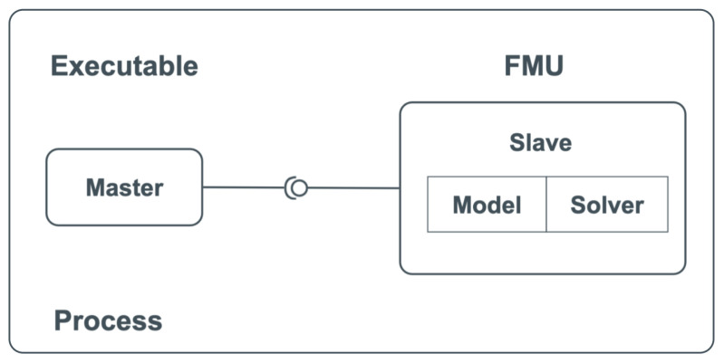
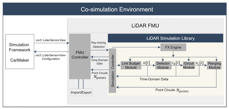
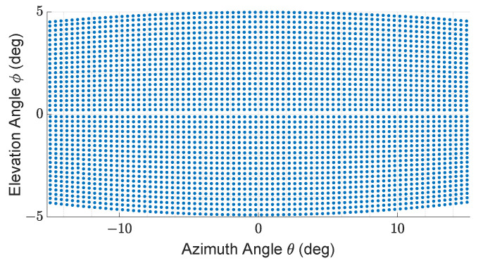
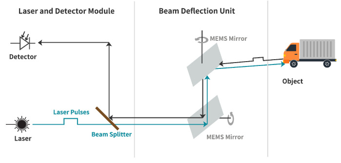
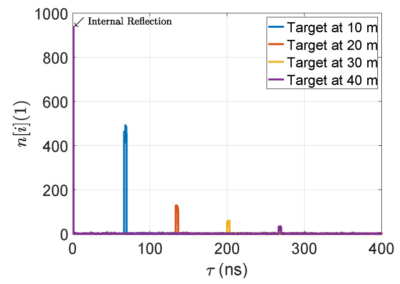
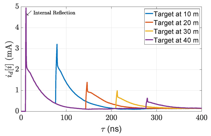
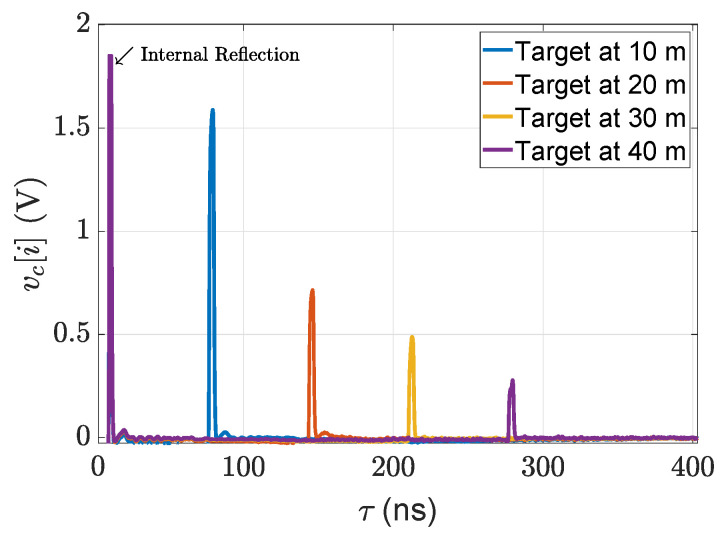
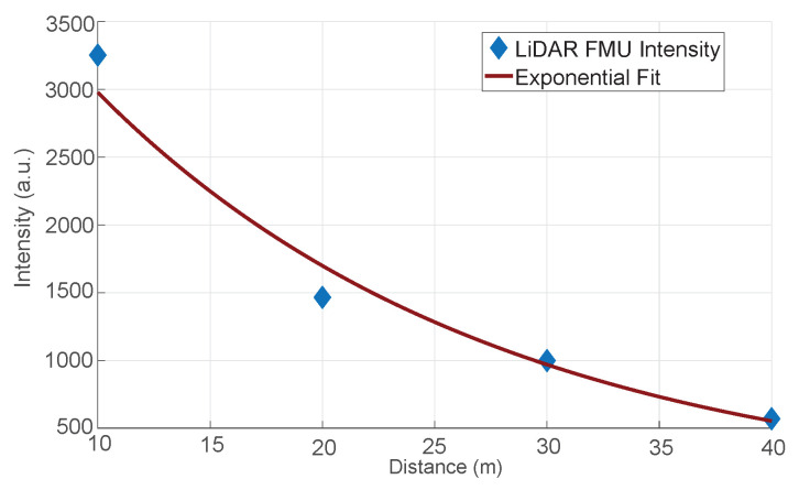
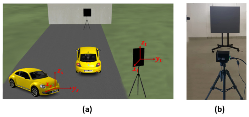
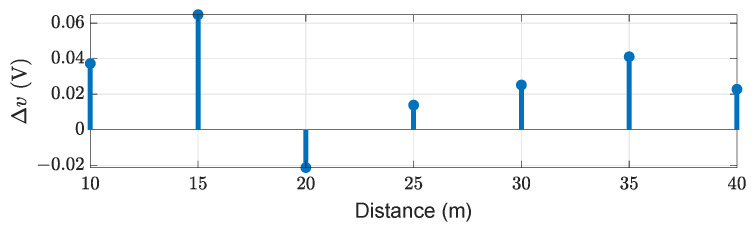
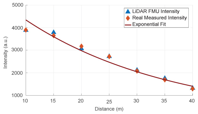
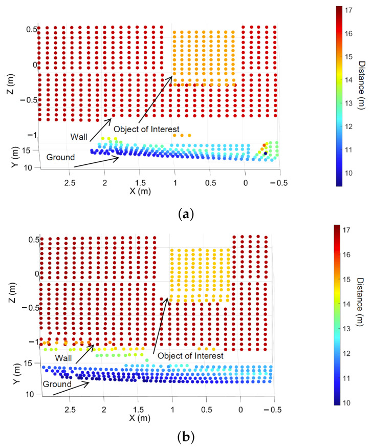
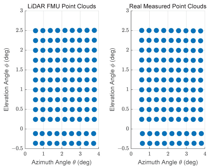
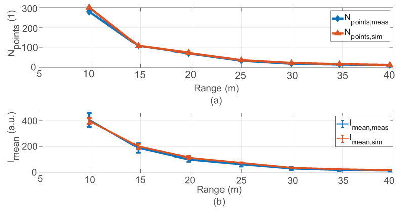
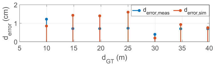
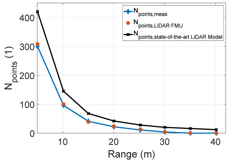
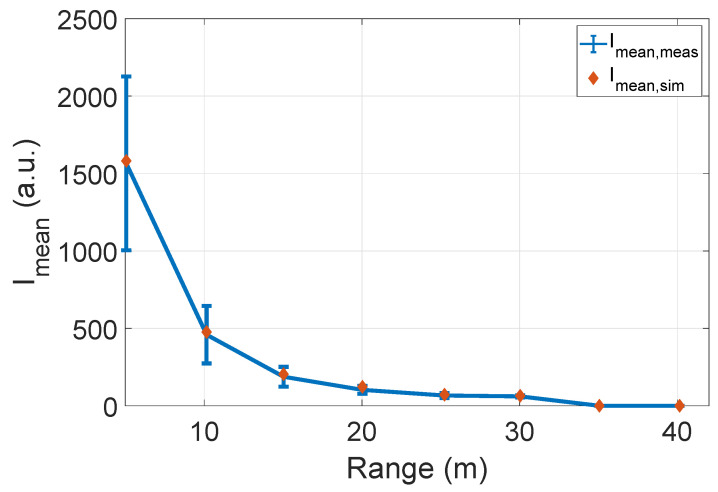
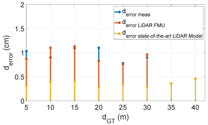
This work introduces a process to develop a tool-independent, high-fidelity, ray tracing-based light detection and ranging (LiDAR) model. This virtual LiDAR sensor includes accurate modeling of the scan pattern and a complete signal processing toolchain of a LiDAR sensor. It is developed as a functional mock-up unit (FMU) by using the standardized open simulation interface (OSI) 3.0.2, and functional mock-up interface (FMI) 2.0. Subsequently, it was integrated into two commercial software virtual environment frameworks to demonstrate its exchangeability. Furthermore, the accuracy of the LiDAR sensor model is validated by comparing the simulation and real measurement data on the time domain and on the point cloud level. The validation results show that the mean absolute percentage error (MAPE) of simulated and measured time domain signal amplitude is 1.7%. In addition, the MAPE of the number of points Npoints and mean intensity Imean values received from the virtual and real targets are 8.5% and 9.3%, respectively. To the author's knowledge, these are the smallest errors reported for the number of received points Npoints and mean intensity Imean values up until now. Moreover, the distance error derror is below the range accuracy of the actual LiDAR sensor, which is 2 cm for this use case. In addition, the proving ground measurement results are compared with the state-of-the-art LiDAR model provided by commercial software and the proposed LiDAR model to measure the presented model fidelity. The results show that the complete signal processing steps and imperfections of real LiDAR sensors need to be considered in the virtual LiDAR to obtain simulation results close to the actual sensor. Such considerable imperfections are optical losses, inherent detector effects, effects generated by the electrical amplification, and noise produced by the sunlight.

Keywords: CarMaker; advanced driver-assistance systems; automotive LiDAR sensor; co-simulation environment; functional mock-up interface; functional mock-up unit; open simulation interface; open standard; point clouds; proving ground; silicon photomultipliers detector; standardized interfaces; time domain signal.


Conflict of interest statement

The authors declare no conflict of interest.

Figures

Figure 1
Figure 1
ADAS functions used in modern vehicles, Source: adapted from [2].
Figure 2
Figure 2
Decrease in road fatalities despite the increase in the number of motor vehicles due to the advances of ADAS in Germany, Source: adapted from [1,3]. ABS, anti-lock braking system; ACC, adaptive cruise control; ESC, electronic stability control; LDW, lane departure warning; PA, parking assistant; TSR, traffic sign recognition.
Figure 3
Figure 3
LiDAR working principle. LiDAR sensor mounted on ego vehicle simultaneously sends and receives the laser light partly reflected from the surface of the target and measures the distance.
Figure 4
Figure 4
Co-simulation stand-alone use case [11].
Figure 5
Figure 5
Co-simulation framework of the LiDAR FMU model.
Figure 6
Figure 6
Specification of scan pattern used by LiDAR FMU model and LiDAR sensor: 30 horizontal and 10 vertical FoV, 80 scan lines, frame mode only up, 0.4 horizontal angle spacing, frame rate 6.7 Hz, maximum detection range is 250 m, and minimum detection range is 4.80 m.
Figure 7
Figure 7
Block diagram of MEMS LiDAR sensor. Source: adapted from [49].
Figure 8
Figure 8
The output of the implemented link budget module for 5% reflective point scatter targets.
Figure 9
Figure 9
The output of the implemented SiPM detector module for 5% reflective point scatter targets.
Figure 10
Figure 10
The output of the circuit module for 5% reflective point scatter targets.
Figure 11
Figure 11
The output of the ranging module for 5% reflective point scatter targets.
Figure 12
Figure 12
(a) Static simulation scene to validate the time domain and point cloud data. (b) Real setup to validate the time domain and point cloud data. The 10% reflective target was placed in front of the sensor at different distances. The coordinates of the actual and simulated sensor and target are the same. The ground truth distance dGT is calculated from the sensor origin to the target center.
Figure 13
Figure 13
LiDAR FMU and real measured TDS comparison. The target peaks and noise levels match well. Furthermore, the LiDAR FMU model provides the same results in AURELION from dSPACE for the time domain signals. We used the osi3::GroundTruth interface to get the target’s position in the virtual environment.
Figure 14
Figure 14
The voltages difference Δv of simulated and measured target peaks.
Figure 15
Figure 15
The validation of the ranging module. The simulated and measured intensities values show good agreement.
Figure 16
Figure 16
Exemplary visualization of the Cartesian point clouds received from all the objects in the FoV of LiDAR FMU and real sensor. (a) The LiDAR FMU 3D Cartesian point clouds. (b) The 3D point clouds of real sensors. It should be noted that the modeled and actual objects’ material properties are different except for the Lambertian target. That’s why the number of points Npoints received from the ground and walls are different in simulation and actual measurement.
Figure 17
Figure 17
Visualization in spherical coordinates of points obtained from the actual and simulated Lambertian plate placed at 15 m. The horizontal spacing between the simulated and measured points is θ=0.4 and vertical spacing is ϕ=0.25.
Figure 18
Figure 18
(a) The number of received points from the object of interest in simulation and real measurement is approximately the same at all distance values. However, a slight mismatch in the number of reflections can be observed because it is impossible to replicate the 100% real-world conditions in the simulation, for instance, ambient light. (b) The mean intensity Imean values show good agreement. It can also be observed that the standard deviation of real measured intensity values is higher than the simulated intensity values because the ambient light condition influences the real measured intensity values.
Figure 19
Figure 19
The distance error is below the range accuracy, that is ±2 cm.
Figure 20
Figure 20
(a) The test vehicle was equipped with a LiDAR sensor and global positioning system (GPS). The GPS ADMA-G-PRO+ from Genesys Inc. is used as the reference sensor with a range accuracy of 0.1 m. The size of the 10% reflective plate is 0.5 × 0.5. (b) The static simulation scene. The ground truth distance dGT is calculated from the sensor reference point to the center of the plate target in simulation and real measurement by using Equation (14).
Figure 21
Figure 21
Specification of scan pattern used by the real and virtual LiDAR sensors for proving ground tests: 42 horizontal and 10 vertical FoV, 40 scan lines, frame mode only up, 0.4 horizontal angle spacing, frame rate 13.3 Hz, maximum detection range is 250 m, and minimum detection range is 4.80 m.
Figure 22
Figure 22
The comparison between the number of received points Npoints obtained from the simulated and real 10% Lambertian plate. The actual measured and LiDAR FMU received point cloud Npoints are similar. However, the number of points Npoints yielded by the state-of-the-art LiDAR sensor model are higher. The MAPE for the number of received Npoints of LiDAR FMU is 9.6% and 48.4% for the state-of-the-art LiDAR sensor model up to 30 m.
Figure 23
Figure 23
The exemplary point clouds provided by real and virtual LiDAR sensor models for 0.5 m × 0.5 m Lambertian plate placed at 30 m. (a) Real measured point clouds (b) LiDAR FMU point clouds (c) State-of-the-art LiDAR sensor model. The real and LiDAR FMU points are noisy and dispersed. However, the state-of-the-art LiDAR model points are ideal and aligned.
Figure 24
Figure 24
The comparison of measured and simulated mean intensity Imean values. The mean intensity Imean values show good agreement. The MAPE for the mean intensity Imean is 11.1%. It should be noted that comparing intensity values of the real measurement and state-of-the-art sensor model is impossible because their units are different.
Figure 25
Figure 25
The distance error derror of real and virtual sensors is below the range accuracy of the real sensor ±2 cm.

References

    1. KBA Bestand Nach Fahrzeugklassen und Aufbauarten. [(accessed on 15 April 2022)]. Available online: https://www.kba.de/DE/Statistik/Fahrzeuge/Bestand/FahrzeugklassenAufbaua....
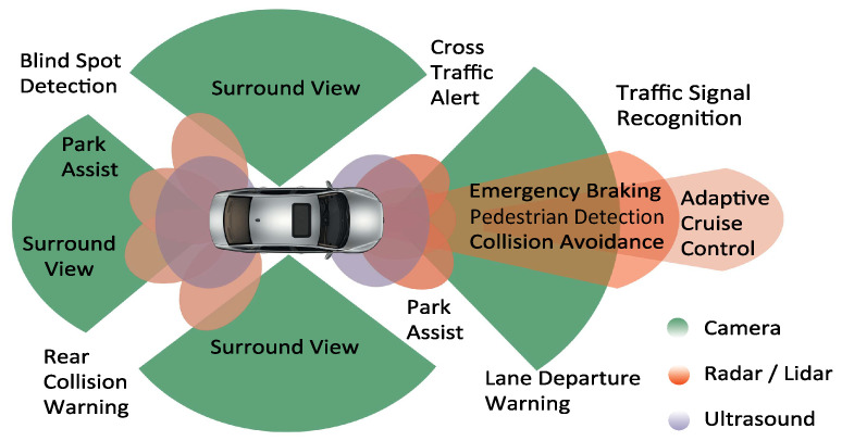
    1. Synopsys What is ADAS? [(accessed on 26 August 2021)]. Available online: https://www.synopsys.com/automotive/what-is-adas.html.
    1. Thomas W. Autonomous Driving. Springer; Berlin/Heidelberg, Germany: 2016. Safety benefits of automated vehicles: Extended findings from accident research for development, validation and testing; pp. 335–364.
    1. Kalra N., Paddock S.M. Driving to safety: How many miles of driving would it take to demonstrate autonomous vehicle reliability? Transp. Res. Part A Policy Pract. 2016;94:182–193. doi: 10.1016/j.tra.2016.09.010. - DOI
    1. Winner H., Hakuli S., Lotz F., Singer C. Handbook of Driver Assistance Systems. Springer International Publishing; Amsterdam, The Netherlands: 2016. pp. 405–430.

LinkOut - more resources