DBSegment: Fast and robust segmentation of deep brain structures considering domain generalization

Abstract

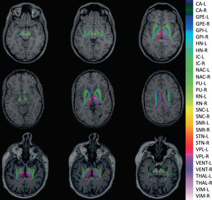
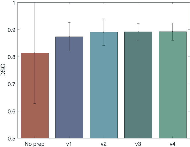
Segmenting deep brain structures from magnetic resonance images is important for patient diagnosis, surgical planning, and research. Most current state-of-the-art solutions follow a segmentation-by-registration approach, where subject magnetic resonance imaging (MRIs) are mapped to a template with well-defined segmentations. However, registration-based pipelines are time-consuming, thus, limiting their clinical use. This paper uses deep learning to provide a one-step, robust, and efficient deep brain segmentation solution directly in the native space. The method consists of a preprocessing step to conform all MRI images to the same orientation, followed by a convolutional neural network using the nnU-Net framework. We use a total of 14 datasets from both research and clinical collections. Of these, seven were used for training and validation and seven were retained for testing. We trained the network to segment 30 deep brain structures, as well as a brain mask, using labels generated from a registration-based approach. We evaluated the generalizability of the network by performing a leave-one-dataset-out cross-validation, and independent testing on unseen datasets. Furthermore, we assessed cross-domain transportability by evaluating the results separately on different domains. We achieved an average dice score similarity of 0.89 ± 0.04 on the test datasets when compared to the registration-based gold standard. On our test system, the computation time decreased from 43 min for a reference registration-based pipeline to 1.3 min. Our proposed method is fast, robust, and generalizes with high reliability. It can be extended to the segmentation of other brain structures. It is publicly available on GitHub, and as a pip package for convenient usage.

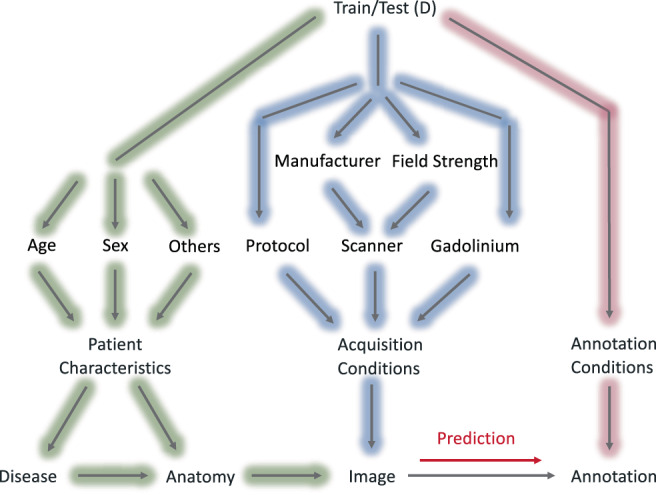
Keywords: confounder; deep brain structures; deep learning; magnetic resonance imaging; segmentation.

FIGURE 1

Deep brain structures segmentation. The segmentation results of the network are shown for one of the test scans. The right and the left hemisphere are visualized with the same color. SNC, SNR, VIM, and VPL are not shown in this figure. The full name of the structures can be found in Table 2

FIGURE 2

The causal diagram of the deep brain structures segmentation workflow. The factors affecting the annotation prediction are categorized to three main groups; patient characteristics (green), acquisition conditions (blue), and annotation conditions (pink)

FIGURE 3

LODO cross‐validation performance. The performance of each fold was measured with DSC on the left out dataset. The average DSC of each subject was calculated for all labels excluding the brain mask and the ventricles. Subjects belonging to the same fold were plotted together. The average DSC of the folds were 0.87 ± 0.03, 0.88 ± 0.03, 0.89 ± 0.03, 0.91 ± 0.01, 0.90 ± 0.02, 0.90 ± 0.03, and 0.86 ± 0.03 on SRH, MIRIAD, ABIDE‐II, PPMI, ADNI, OASIS3, and HCP datasets respectively

FIGURE 4

LODO cross‐validation performance on each label. On the top, the DSC of each label was measured for all the training subjects during LODO cross‐validation. Similarly, on the bottom, the AHD is measured. To visualize both the variability between different structures at lower AHD and the outliers at higher AHD values, the plot has two scales, below between 0 and 1 and on top between 1 and 9 and 1 and 10. The full name of the labels can be find in Table 2. The exact mean values of the DSC and the ADH are given in table S5

FIGURE 5

The network's performance on the unseen datasets (test sets). The average DSC of each subject was calculated for all its labels (all brain structures, without brain mask and the ventricles). The subjects belonging to the same dataset were plotted together. The average DSC of the datasets were 0.90 ± 0.02, 0.88 ± 0.02, 0.91 ± 0.01, 0.91 ± 0.02, 0.88 ± 0.03, 0.79 ± 0.06 and 0.87 ± 0.06 for IXI, UNC, LA5C, THP, AUH, CHL, and CUB respectively

FIGURE 6

The network's performance on each label of the unseen datasets (test sets). On the top, the DSC of each label was measured across all the test subjects. Similarly, on the bottom, the AHD is measured. To visualize both the variability between different structures at lower AHD and the outliers at higher AHD values, the plot has two scales, below between 0 and 1 and on top between 1 and 5, and 1 and 9. The full name of the labels can be find in Table 2. The exact mean values of the DSC and the ADH are given in table S5

FIGURE 7

Examples of DBSegment outputs. Three random images from the test set are plotted with the segmentation out of DBSegment (rows). Three 2D slices are shown to for each subject (columns). Visible structures: Top right: IC, SNC, SNR, RN, top middle: STN, IC, RN, slightly visible: VENT, THAL, NAC, PU, top left: HN, THAL, VIM, VPL, IC, GPI, GPE, PU, NAC, VENT, middle right: IC, SNC, SNR, slightly visible: NAC, middle: THAL, VIM, VPL, HN, VENT, IC, PU, CA, GPE, slightly visible: GPI, middle left: VENT, CA, IC, bottom right: THAL, VIM, VPL, IC, VENT, PU, slightly visible: GPE, GPI, Bottom middle: THAL, HN, VPL, STN, IC, PU, slightly visible: VIM, GPE, bottom right: IC, SNC, SNR, VENT, RN, slightly visible: THAL, CA

FIGURE 8

Analysis of DSC stratified by potential confounding factors. The factors were obtained from the causal diagram (Figure 2). Top row ‐ blue: Factors affecting the acquisition conditions. Protocol: MPRAGE with the mean DSC = 0.90 ± 0.03, FSPGR, mean DSC = 0.88 ± 0.04, and FLASH, mean DSC = 0.89 ± 0.02, scanner: Siemens (SM) 1.5 T, mean DSC = 0.90 ± 0.02, SM 3 T, mean DSC = 0.89 ± 0.03, Philips (PL) 1.5 T, mean DSC = 0.91 ± 0.01, PL 3 T, mean DSC = 0.89 ± 0.03, General Electric (GE) 1.5 T, mean DSC = 0.89 ± 0.03, and GE 3 T, mean DSC = 0.88 ± 0.05, gadolinium: Images without gadolinium enhancement (No Gado), mean DSC = 0.90 ± 0.03, and images with gadolinium enhancement (Gado), mean DSC = 0.82 ± 0.06. Bottom row ‐ green: Factors affecting the patient's characteristics. Disease: Healthy, mean DSC = 0.89 '± 0.03, neurodegenerative disorders (NDD), including, Alzheimer's disease, dementia, memory concern, cognitive impairment, Parkinson's disease, and early stage Parkinson's disease, essential tremor, and dystonia, mean DSC = 0.89 ± 0.04, psychiatric disorders (PSD), including bipolar disorder, schizophrenia, and attention deficit hyperactivity disorder, mean DSC = 0.91 ± 0.01, and others, including, epilepsy, autism, trauma, and pain, mean DSC = 0.88 ± 0.04. Age: Below and equal to 20, mean DSC = 0.89 ± 0.03, between 20 and 40 and equal to 40 (20–40), mean DSC = 0.89 ± 0.03, similarly 40–60, mean DSC = 0.89±0.03, 60–80, mean DSC = 0.90 ± 0.03, and above 80, mean DSC = 0.89 ± 0.03. Sex: Female, mean DSC = 0.90 ± 0.03, and male, mean DSC = 0.89 ± 0.03. The size of each class in the training set (Tr), and the test set (Ts) are shown on the bottom of the plots

FIGURE 9

Results of the ablation study on the preprocessing steps. The DSC performance of five networks with different preprocessing steps are presented for all cross‐validation data. Standard deviations across subjects are presented on top of the bar plots. The first network is not using any preprocessing. The second network, builds on the V1 preprocessing, conforming all MR images to the same orientation. For the V2 preprocessing, all MR images were conformed to the same orientation and 1 × 1 × 1 mm voxel spacing, in V3, MR images were conformed to the same orientation, 1 × 1 × 1 mm voxel spacing and 256 × 256 × 256 dimension, in V4, MR images were conformed to the same orientation, 1 × 1 × 1 mm voxel spacing, 256 × 256 × 256 dimension, and the intensity range of each image was normalized between 0 and 255

FIGURE 10

The DSC between the network and the gold standard brain mask. The DSC is plotted for all the cross‐validation subjects (BM‐CV), and all the test subjects (BM‐test)

References

-
- Abelson, J. L. , Curtis, G. C. , Sagher, O. , Albucher, R. C. , Harrigan, M. , Taylor, S. F. , Martis, B. , & Giordani, B. (2005). Deep brain stimulation for refractory obsessive‐compulsive disorder. Biological Psychiatry, 57(5), 510–516. - PubMed
- Aleksovski, D. , Miljkovic, D. , Bravi, D. , & Antonini, A. (2018). Disease progression in Parkinson subtypes: The PPMI dataset. Neurological Sciences, 39(11), 1971–1976. - PubMed
- Anderson, D. N. , Osting, B. , Vorwerk, J. , Dorval, A. D. , & Butson, C. R. (2018). Optimized programming algorithm for cylindrical and directional deep brain stimulation electrodes. Journal of Neural Engineering, 15(2), 26005. - PubMed
- Andersson, J. L. R. , Jenkinson, M. , and Smith, S. (2010). Non‐linear registration, aka spatial normalization (FMRIB Technical Report TR07JA2).
Publication types
MeSH terms
Grants and funding
LinkOut - more resources
Full Text Sources