. 2022 Nov;19(11):1438-1448.
doi: 10.1038/s41592-022-01639-4. Epub 2022 Oct 17.

Omnipose: a high-precision morphology-independent solution for bacterial cell segmentation

Affiliations

Omnipose: a high-precision morphology-independent solution for bacterial cell segmentation

Kevin J Cutler et al. Nat Methods. 2022 Nov.

Abstract

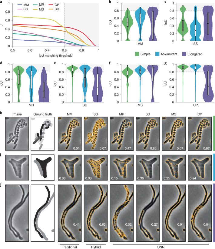
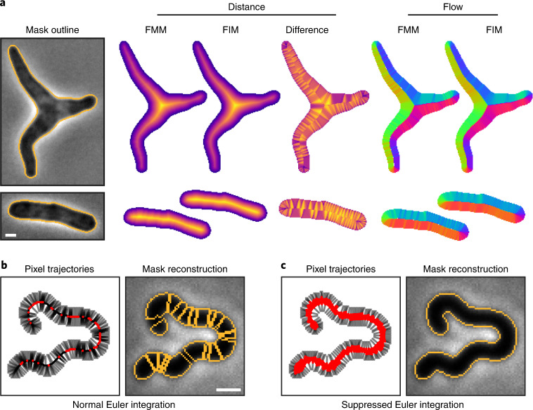
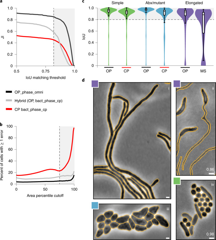
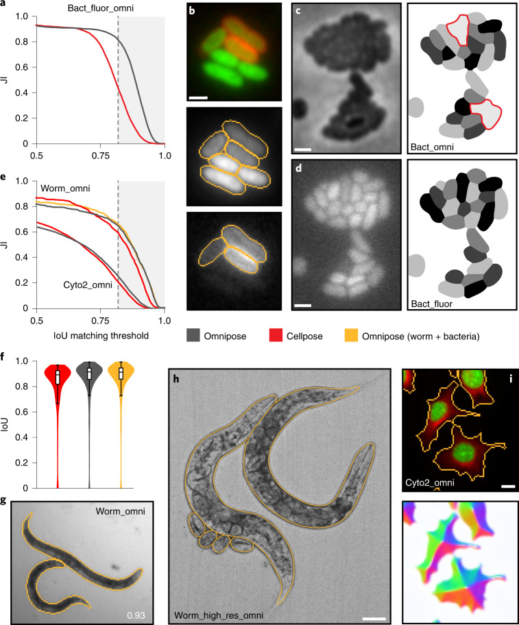
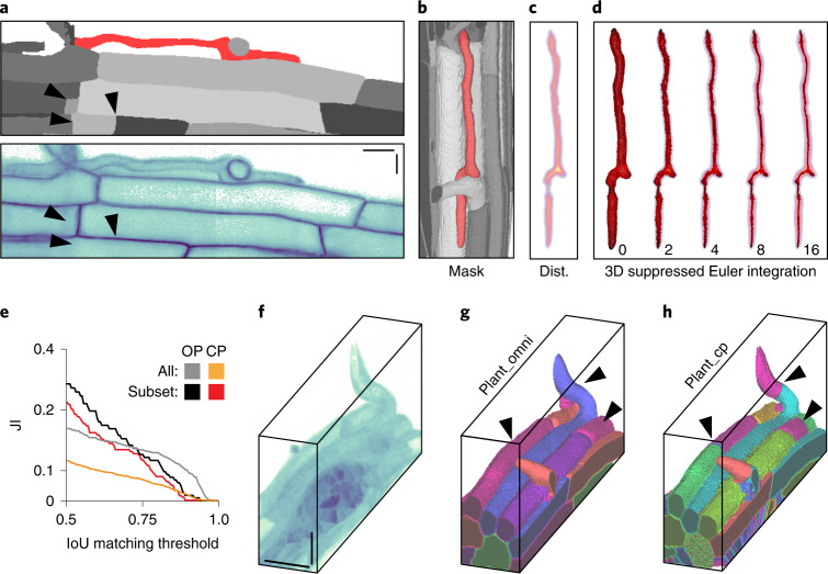
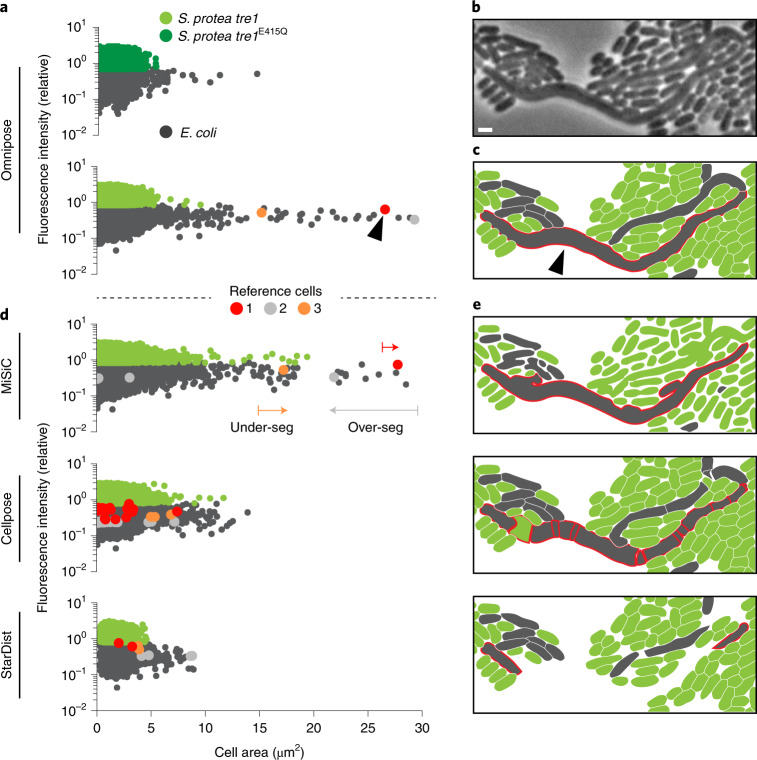
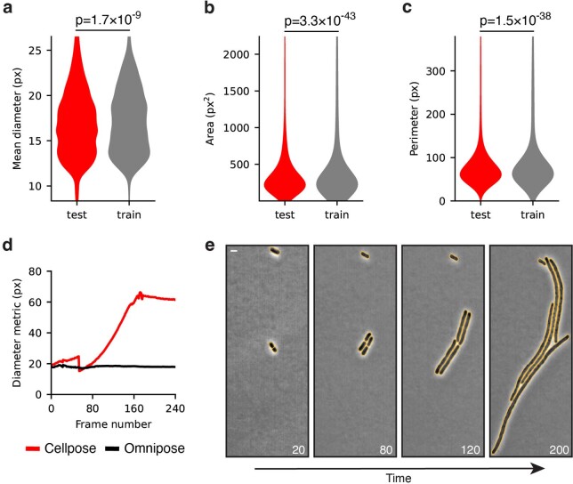
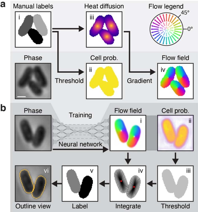
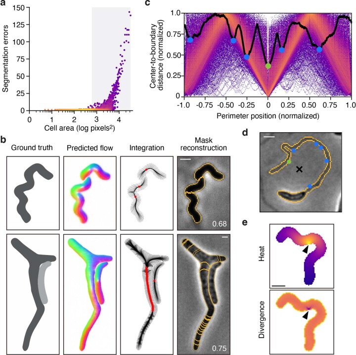
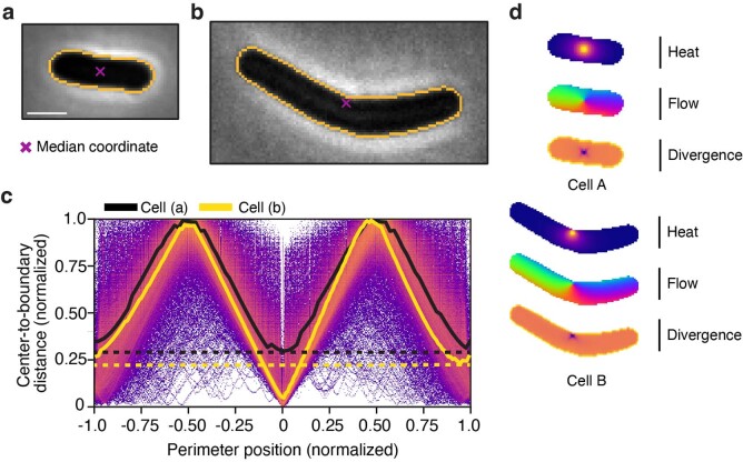
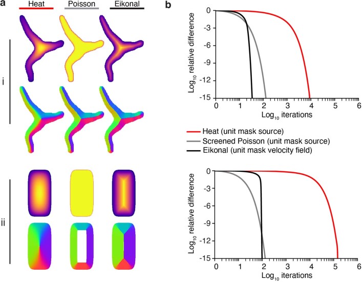
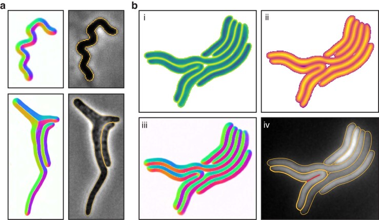
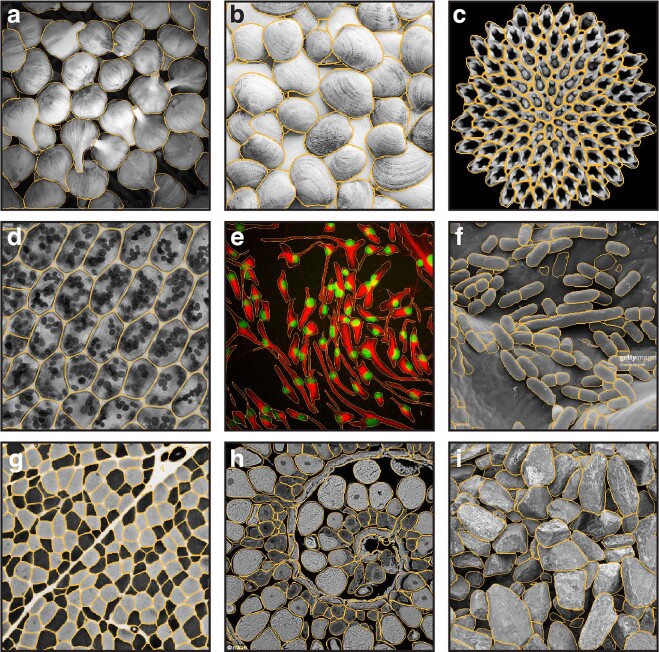
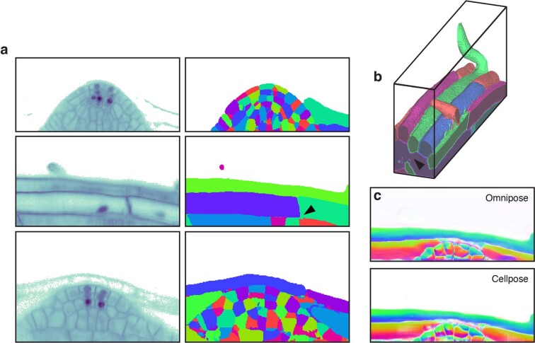
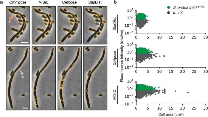
Advances in microscopy hold great promise for allowing quantitative and precise measurement of morphological and molecular phenomena at the single-cell level in bacteria; however, the potential of this approach is ultimately limited by the availability of methods to faithfully segment cells independent of their morphological or optical characteristics. Here, we present Omnipose, a deep neural network image-segmentation algorithm. Unique network outputs such as the gradient of the distance field allow Omnipose to accurately segment cells on which current algorithms, including its predecessor, Cellpose, produce errors. We show that Omnipose achieves unprecedented segmentation performance on mixed bacterial cultures, antibiotic-treated cells and cells of elongated or branched morphology. Furthermore, the benefits of Omnipose extend to non-bacterial subjects, varied imaging modalities and three-dimensional objects. Finally, we demonstrate the utility of Omnipose in the characterization of extreme morphological phenotypes that arise during interbacterial antagonism. Our results distinguish Omnipose as a powerful tool for characterizing diverse and arbitrarily shaped cell types from imaging data.


Conflict of interest statement

The authors declare no competing interests.

Figures

Fig. 1
Fig. 1. Quantitative comparison of segmentation methods distinguishes Cellpose as a high-performing algorithm.
a–g, Comparison of segmentation algorithm performance on our bact_phase test dataset (n = 19,538 cells). Overall performance measured by JI (a). MM, Morphometrics; MR, Mask R-CNN; CP, Cellpose; SS, SuperSegger; MS, MiSiC; SD, StarDist. The JI was calculated at the image level and values averaged across the dataset are displayed. Algorithm performance was partitioned by cell type (simple, n = 12,869; Abx/mutant, n = 6,138; elongated, n = 531) (b–g). Images were sorted into types as defined in Supplementary Table 1. Abx, antibiotic. Boxes are centered on medians from Q1 to Q3, whiskers from Q1 − 1.5 IQR to Q3 + 1.5 IQR. IQR, interquartile range Q3–Q1. h–j, Representative micrographs of cell type partitions analyzed in bg, indicated by vertical bars on right. Ground-truth masks and predicted mask outlines generated by the indicated algorithm are displayed. Mean matched IoU values for cells shown are displayed within each micrograph. Bacteria displayed are Vibriocholerae, Pseudomonasaeruginosa, Bacillussubtilis, and Staphylococcusaureus (h), aztreonam-treated E.coli CS703-1 (i), and Streptomycespristinaespiralis (j). All images are scaled equivalently. Scale bar, 1 μm.
Fig. 2
Fig. 2. Core innovations of Omnipose.
a, Comparison of distance field algorithms and corresponding flow fields on ground-truth masks. FMM produces ridges in the distance field resulting from pixelation on the cell mask boundary. Our smooth FIM algorithm minimizes these features. The difference image (FIM − FMM) highlights artifacts in the FMM method. Flow fields are calculated as the normalized gradient of the distance field. Boundary pixelation affects the FMM flow field deep into the cell, regardless of cell size. b,c, Comparison of mask reconstruction algorithms on a smooth flow field. Boundary pixel trajectories and resulting mask outlines from standard Euler integration (b). Trajectories and mask outlines under suppressed Euler integration (c). Red dots indicate the final positions of all cell pixels, not only the boundary pixels for which trajectories are displayed. Bacteria displayed are E.coli CS703-1 (a) and H.pylori (b,c) both treated with aztreonam. Scale bars, 1 μm. Images are representative of 1,299 E.coli and 701 H.pylori cells in the total ground-truth dataset, respectively.
Fig. 3
Fig. 3. Omnipose substantially outperforms Cellpose on elongated cells.
a, Overall performance of Omnipose (OP) (bact_phase_omni) and Cellpose (CP) (bact_phase_cp) measured by JI. The hybrid method (gray) uses the original center-seeking flow output of bact_phase_cp and the mask reconstruction of Omnipose. Gray box represents IoU ≥ 0.8. n = 19,570 cells in the test set. b, Quantification of segmentation performance by cell size. The percent of cells with at least one segmentation error is computed for cells in each area percentile group from 1 to 100. Gray box represents the top quartile. c, Omnipose IoU distribution on the bact_phase dataset compared to the next highest performing algorithm in each of three cell categories (simple, n = 12,869; Abx/mutant, n = 6,138; and elongated, n = 531). Boxes centered on medians from Q1 to Q3, whiskers from Q1 − 1.5 IQR to Q3 + 1.5 IQR. d, Example micrographs and Omnipose segmentation. Mean matched IoU values shown. Bacteria displayed are Streptomycespristinaespiralis (i), Caulobactercrescentus grown in HIGG medium (ii), Shigellaflexneri treated with A22 (iii) and a mix of Pseudomonasaeruginosa, Staphylococcusaureus, V.cholerae, and Bacillussubtilis (iv). HIGG, Hutner base–imidazole-buffered glucose–glutamate. Scale bars, 1 μm.
Fig. 4
Fig. 4. Omnipose models trained and evaluated on assorted imaging modalities and subjects.
Relevant Omnipose model names are provided (also Supplementary Table 2). a, Performance of bacterial fluorescence Omnipose (bact_fluor_omni) and Cellpose (bact_fluor_cp) models. Test set consists of n = 14,587 cells. b, Fluorescence micrograph (top) and corresponding bact_fluor_omni segmentation results of B.thailandensis expressing cytoplasmic green fluorescent protein (GFP) (segmentation, middle) or outer-membrane localized mCherry (segmentation, bottom). c,d, Francisellatularensis subsp novicida segmentation using bact_phase_omni (c) or bact_fluor_omni (d) Omnipose models. Two notable bact_phase_omni segmentation errors are highlighted in red. Scale bars, 1 μm. e, Performance of Omnipose models trained on cyto2 (cyto2_omni, n = 10,232) and C.elegans (worm_omni) datasets versus corresponding Cellpose models. Results for Omnipose and Cellpose trained on either C.elegans alone (gray, red) or Omnipose on C.elegans and bacterial data (yellow) are shown. Cyto2 test dataset, n = 10,232 cells. C.elegans test dataset, n = 1,264 worms. f, IoU distribution for the masks predicted by each method on our C.elegans test dataset (n = 1,264). Boxes centered on medians from Q1 to Q3, whiskers from Q1 − 1.5 IQR to Q3 + 1.5 IQR. g, Example segmentation of C.elegans in the BBBC010 dataset used in e,f. IoU score shown. Scale bar, unavailable. h, Example segmentation of high-resolution C.elegans (minimum projection brightfield). Scale bar, 50 μm. i, Example multi-channel Omnipose segmentation in the cyto2 dataset. Scale bar, 3 μm.
Fig. 5
Fig. 5. Omnipose can be applied to 3D datasets.
a, Volume slice in the A.thaliana 3D training set. Black arrows denote over-segmentation in the ground truth labels. Red corresponds to the cell in bd. b, Selected cell in context of ground-truth data. c, Ground-truth distance field for selected cell in b. d, Steps of the suppressed Euler integration for selected cell in b. Boundary pixels shown, colored by overall displacement (dark to light red). e, Performance of Omnipose (OP, plant_omni) and Cellpose (CP, plant_cp) on the full test dataset (n = 604) and on a subset without excluded regions (Methods) depicted in fh (n = 73). f–h, Ground-truth masks (f) and segmentation results of A.thaliana using Omnipose (g) and Cellpose (h). Scale bars, 20 μM.
Fig. 6
Fig. 6. Omnipose facilitates the accurate identification of intoxicated E.coli cells.
a, Fluorescence/area population profile according to Omnipose segmentation (bact_phase_omni) in control and experimental conditions. K-means clustering on GFP fluorescence distinguishes S.proteamaculans tre1/tre1E415Q (light/dark green markers) from E.coli (gray markers). n = 209,000 cells in experimental population (S.proteamaculans tre1) and n = 85,260 cells in control group (S.proteamaculans tre1E415Q). b, Example of extreme filamentation of E.coli in response to active Tre1. c, Omnipose accurately segments all cells in the image. Largest cell indicated with black arrow. d, MiSiC predicts large cell masks over both species. Cellpose (bact_phase_cp) and StarDist fail to predict any cells above 15 μm2. e, Example segmentation results highlighting typical errors encountered with MiSiC (under-segmentation), Cellpose (over-segmentation) and StarDist (incomplete masks). Mask mergers cause some E.coli to be misclassified as S.proteamaculans. Scale bar, 1 μm.
Extended Data Fig. 1
Extended Data Fig. 1. Size and morphology metrics are indistinguishable between cell populations included in training and test datasets.
(a) Mean cell diameter, (b) cell area, and (c) cell perimeter calculated for our bacterial phase-contrast ground-truth dataset. P-values are displayed for the two-sided KS test. n = 47,000 (27,500 for training, 19,500 for testing). (d). Comparison of diameter metrics of a timelapse of elongated cell growth. The Cellpose diameter metric is the diameter of a circle with equivalent area. Omnipose diameter metric is proportional to the mean of the distance transform (see Methods). (e) Bacteria displayed are a single population analyzed of A. baylyi transformed with a ΔftsN::kan PCR fragment. Yellow lines indicate cell label boundaries. Scale bar is 1 μm.
Extended Data Fig. 2
Extended Data Fig. 2. The relationship between IoU and segmentation accuracy.
(a) Illustration of 0–12 pixel displacement of cell mask (red outline) and corresponding IoU values using a synthetic cell of typical bacterial size and resolution (solid black). (b) Quantification of the impact of mask shift on IoU values, determined using the synthetic cell shown in (a).
Extended Data Fig. 3
Extended Data Fig. 3. Details of the Cellpose algorithm.
(a) Stages of the Cellpose training pipeline. Ground truth masks (i) are converted to cell probability (ii) by binary thresholding and a heat distribution (iii) by simulated diffusion from the median pixel coordinate. The flow field (iv) is defined by the normalized gradient of (iii). Color-magnitude representations of this vector field follow the flow legend diagram. The phase, cell probability and flow fields are used to train the network. (b) Stages of the cellpose prediction pipeline. Phase images are processed by the trained cellpose network into the intermediate flow field and cell probability outputs (i-ii). A binary threshold is applied to the probability to identify cell pixels (iii). Pixels are Euler-integrated under the flow field until they converge at common points. Boundary pixel trajectories are depicted in iv. Each pixel is assigned a unique label corresponding to the center to which it converged (v). This segmentation result is commonly depicted in an outline view (vi). Bacteria shown are Escherichia coli. Scale bar is 1 μm.
Extended Data Fig. 4
Extended Data Fig. 4. Cellpose over-segments extended, anisotropic cells.
(a) Single-cell analysis of Cellpose segmentation error as a function of cell area. Color represents density on a log scale. Gray box represents the top quartile of cell areas (n = 19,570). (b) Example images representative of 1,128 cells with segmentation errors in the top area quartile (n = 4,887). Corresponding boundary pixel trajectories are shown in black and final pixel locations in red. Predicted mask overlays are shown with mean matched IoU values. Cellpose model bact_phase_cp used in (a,b). (c) Analysis of stochastic center-to-boundary distances in our ground-truth dataset. Distance from the center (median pixel coordinate) to each boundary pixel is normalized to a maximum of 1. Position along the boundary is normalized from −1 to 1 and centered on the point closest to the median pixel. Center-to-boundary for the cell in (d) is highlighted in black. (d) Representative cell with median coordinate outside the cell body (black X). Cellpose projects this point to the global minima of this function (green dot), but several other local minima exist (blue dots). (e) The heat distribution resulting from a projected cell center (black arrow). The normalized gradient corresponds to the divergence shown. (d-e) represent n = 617 cells with projected centers in the training dataset. Bacteria displayed are (a,e) Helicobacter pylori, (b) Escherichia coli CS703-1, both treated with aztreonam and (d) Caulobacter crescentus grown in HIGG media. Scale bars, 1 μm.
Extended Data Fig. 5
Extended Data Fig. 5. Median coordinates used to generate Cellpose ground-truth flow fields are asymmetrically localized for some bacterial cell morphologies.
(a) Rod-shaped E. coli with symmetric median coordinate. Symmetry of the center is reflected in A by equal high and low points corresponding to the extremal points along the long and short axes of the cell. (b) Curved B. subtilis with median coordinate asymmetrically close to the cell boundary. This asymmetry is reflected in A by a secondary minimum above the global minimum corresponding to the diametrically opposing point along the short axis of the cell. (c) Center-to-boundary distance highlighted for cells A (black) and B (yellow) with non-projected median coordinates. Dashed lines indicate the larger of the two minima along the medial axis. (d) Flow fields generated by Cellpose for cells A and B. Scale bar is 1 μm. Images scaled equivalently.
Extended Data Fig. 6
Extended Data Fig. 6. The Eikonal equation provides a fast and accurate flow field calculation for diverse cell morphologies and sizes.
(a) Partial differential equation solutions (top rows) and corresponding flow fields (bottoms rows) calculated for two examples cells (i, ii) using a relaxation algorithm for the heat, Poisson and Eikonal equations. Cell (i) is drawn from our dataset (mean diameter 37px) and cell (ii) is a synthetic rod-shaped cell (mean diameter 192px). (b) Convergence measured by the average difference at each iteration (maximum normalized to 1) for cells (i,ii).
Extended Data Fig. 7
Extended Data Fig. 7. Omnipose output on diverse morphologies.
(a) Omnipose flow and segmentation corresponding to the cells of Extended Data Fig. 4b. (b) (i-iii) Boundary, distance and flow output using bact_fluor_omni model on S. flexneri treated with cephalexin. (iv) Overlaid mask outlines. The cell in bold yellow is missing the self-contact boundary in red.
Extended Data Fig. 8
Extended Data Fig. 8. Omnipose accurately segments diverse images from the cyto2 test dataset.
(a-i) Selection of images from the cyto2 test dataset with superimposed outlines representing Omnipose cyto2_omni model segmentation. Subjects are not defined, as the cyto2 dataset lacks metadata and is comprised of anonymized contributions.
Extended Data Fig. 9
Extended Data Fig. 9. Errors in the three-dimensional A. thaliana ground-truth dataset impact training and performance metrics of Ominpose and Cellpose.
(a) Slices of ground truth training set volumes. Images show errant pixels and apparent flaws in ground truth masks. Black arrow indicates one instance of a joined mask. (b) Ground truth masks for the test volume in Fig. 5e-h. Two cells are joined under one label (black arrow). (c) Slices of the predicted Omnipose and Cellpose flow fields through the middle of the volume in (b).
Extended Data Fig. 10
Extended Data Fig. 10. Example segmentation errors by StarDist, Cellpose and MiSiC of E. coli cells undergoing intoxication by S. proteamaculans Tre1.
(a) Examples of segmentation failures demonstrated by each method. Cells 2 and 3 indicated with orange and gray arrows are the reference cells highlighted in Fig. 6a, d. Scale bars are 1 μm. (b) Control populations segmented by StarDist, Cellpose and MiSiC. Notably, Cellpose and MiSiC exhibit an enrichment of larger cells even in the control, a consequence of both under-segmented (merged) cells as well as fragments of over-segmented large cells.

References

    1. Jeckel, H. & Drescher, K. Advances and opportunities in image analysis of bacterial cells and communities. FEMS Microbiol Rev10.1093/femsre/fuaa062 (2021). - PMC - PubMed
    1. Bali, A. & Singh, S. N. A review on the strategies and techniques of image segmentation. In 2015 Fifth International Conference on Advanced Computing & Communication Technologies 113–120 (2015).
    1. Lucas AM, et al. Open-source deep-learning software for bioimage segmentation. Mol. Biol. Cell. 2021;32:823–829. - PMC - PubMed
    1. Kysela DT, Randich AM, Caccamo PD, Brun YV. Diversity takes shape: understanding the mechanistic and adaptive basis of bacterial morphology. PLoS Biol. 2016;14:e1002565. - PMC - PubMed
    1. Jones SE, Elliot MA. ‘Exploring’ the regulation of Streptomyces growth and development. Curr. Opin. Microbiol. 2018;42:25–30. - PubMed

Publication types

LinkOut - more resources