Estimation of skeletal kinematics in freely moving rodents

Abstract

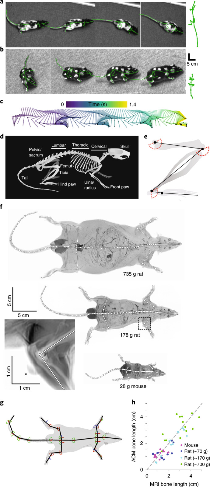
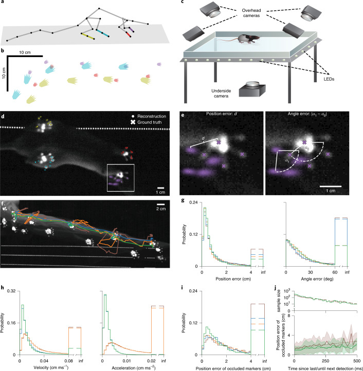
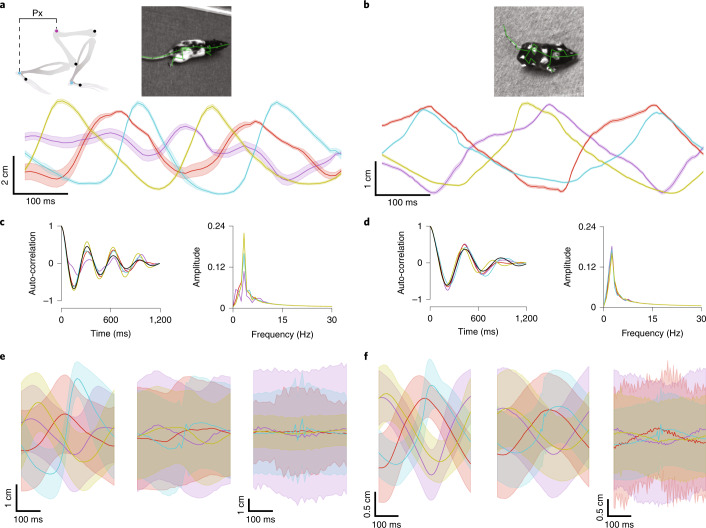
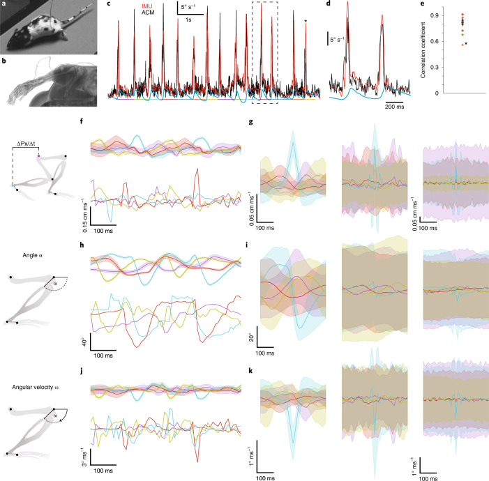
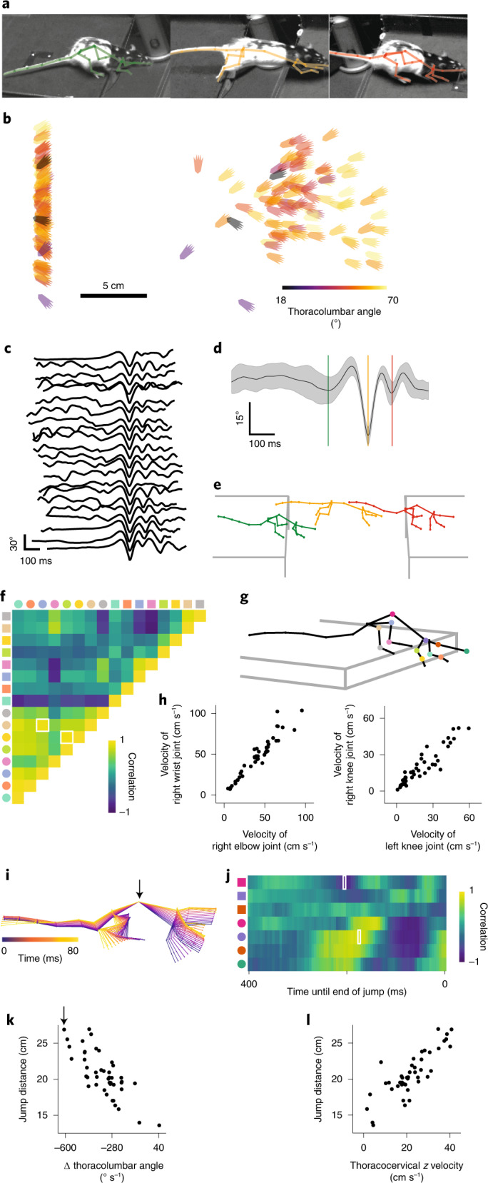
Forming a complete picture of the relationship between neural activity and skeletal kinematics requires quantification of skeletal joint biomechanics during free behavior; however, without detailed knowledge of the underlying skeletal motion, inferring limb kinematics using surface-tracking approaches is difficult, especially for animals where the relationship between the surface and underlying skeleton changes during motion. Here we developed a videography-based method enabling detailed three-dimensional kinematic quantification of an anatomically defined skeleton in untethered freely behaving rats and mice. This skeleton-based model was constrained using anatomical principles and joint motion limits and provided skeletal pose estimates for a range of body sizes, even when limbs were occluded. Model-inferred limb positions and joint kinematics during gait and gap-crossing behaviors were verified by direct measurement of either limb placement or limb kinematics using inertial measurement units. Together we show that complex decision-making behaviors can be accurately reconstructed at the level of skeletal kinematics using our anatomically constrained model.

Fig. 1. Learning an anatomically constrained skeleton model for mice and rats.

a, Example images of a freely moving rat with painted surface labels, also showing the fitted and re-projected skeleton model (green). Scaled skeleton shown at right for comparison with b. b, as for a, but showing images from a freely moving mouse. Scaled skeleton on right for comparison with a. c, Time series of the reconstructed right hind limb during the sequence shown in a. d, Schematic image of a rat skeleton showing anatomical landmarks. e, Schematic image of a hind limb with modeled bones (black lines) and joints (black dots) as well as enforced joint angle limits for flexion and extension (red dashed lines). f, MRI scans (maximum projection) of two rats of different weights (top, middle), a mouse (bottom) and an enlargement of the right elbow joint from a rat (bottom left, mean projection, area denoted by dashed box) with manually labeled bone (white lines) and joint (white dots) positions. Note visible MRI surface marker (asterisk). g, 3D representation of a rat’s MRI scan showing the animal’s surface (gray) and the aligned skeleton model (black lines) and joint angle limits for flexion or extension (red lines), abduction or adduction (green lines) and internal or external rotation (blue lines). h, Learned bone lengths compared to MRI bone lengths (n = 6 rats and 2 mice). Colors represent mouse data (magenta) and small (blue, 71 g and 72 g), medium (cyan, 174 g and 178 g) and large (green, 699 g and 735 g) rat data.

Fig. 2. Comparison between inferred and measured paw positions during free behavior.

a, Reconstructed animal pose based on a learned skeleton model with highlighted left front (purple), right front (red), left hind (cyan) and right hind paw (yellow). b, Reconstructed x–y positions of the paws during gait. Colors as in a. c, Schematic image of the FTIR touch-sensing setup with one underneath and four overhead cameras. d, Single image from the underneath camera with reconstructed (x) and ground-truth (filled circle) x–y positions of the paw’s centers and fingers/toes for all four paws. Colors as in a. Large point clouds around landmark locations indicate high uncertainty. Note that only the second toe and finger are represented in the model skeleton, but that the positions of three toes and fingers were detected and tracked. e, Enlarged view of the left front paw in d (white box) showing calculation of position error (left) and the angle error (right). Scale bar in right image applies to both images in e. f, Maximum intensity projection from the underneath camera of a 2.5-s long sequence with trajectories for the reconstructed x–y positions of the right hind paw using the ACM (green), temporal (blue), joint angle (orange) and naive skeleton (brown) models. g, Probability histograms for paw position (left) and angle errors (right) comparing different model constraint regimes. Color-coding as in f. h, Probability histograms for paw velocities (left) and accelerations (right) comparing different model constraint regimes. Color-coding as in f. i, Probability histograms for paw position errors when only undetected surface markers are used for the calculation comparing different model constraint regimes. Color-coding as in f. j, Position errors of occluded markers (bottom, mean ± s.d. of samples) and corresponding binned sample sizes (top) as a function of time since last or until next marker detection comparing different model constraint regimes. Color-coding as in f. Sample sizes differ depending on whether reconstructed poses were obtained via the unscented RTS smoother (green) or not (brown).

Fig. 3. Periodic gait cycles in freely moving rats and mice.

a, Trajectories in the freely moving rat of the normalized x position (Px) as a function of time (mean ± s.d. of 1,000 propagations through the probabilistic model) for the left wrist (purple), right wrist (red), left ankle (cyan) and right ankle (yellow) joint during gait. Schematic above at left illustrates the normalized position of an ankle joint (cyan spot) and normalization joint (magenta). Individual traces show the estimated position (solid line) with the uncertainty in the position represented by the width of the surrounding shaded area. Note that the left and right wrist joints were occluded for large parts of this segment, illustrated by the larger uncertainty in position on these traces. b, As in a, but for data from a freely moving mouse. All joints are clearly visible throughout the mouse segment, resulting in small uncertainty ranges for all traces. c, Autocorrelations of the normalized x position for data from a freely moving rat as a function of time (left) for four different limbs as well as a corresponding model fit via a damped sinusoid (black). Fourier-transformed autocorrelations of all limbs (right) have their maximum peak at the same frequency. Colors as in a. d, As in c, but for data from a freely moving mouse. e, Population-averaged trajectories of the normalized x position for data from freely moving rats as a function of time for the ACM (left), the naive skeleton model (center) and the surface model (right). Individual traces represent mean and s.d. Data from 28 sequences, 146.5 s, 58,600 frames in total from four cameras, n = 2 rats. Colors as in a. Trajectories of the ACM and the naive skeleton model correspond to the 3D joint locations, whereas trajectories of the surface model correspond to the 3D locations of the associated surface markers. Scale bar on left applies to both left and center. f, As in e, but for data from freely moving mice. Data from 29 sequences, 93.8 s, 73,536 frames total from four cameras, n = 2 mice. Scale bar on left applies to both left and center.

Fig. 4. 3D pose reconstruction of gait cycles with independent gyroscope-based verification.

a, Overhead camera image of freely moving rat with attached IMUs and signal wires. b, MicroCT image of IMU unit placed on skin over tibia. c, Example traces of inferred absolute angular velocity of the leg from the ACM (black), the angular velocity directly measured by the IMU (red) and left ankle x position (blue, anatomical position as in f). Colored line segments below the traces illustrate the segments used for correlation calculations in e. Asterisk marks the peak that corresponds to the lowest correlation value in e. Dashed box shown expanded in d. e, Correlation coefficients between simultaneously recorded ACM (black in c) and IMU (red in c) traces around peaks (colored segments in c) (14 peaks, rat 1, red) and for data from a second rat (blue, 6 peaks). Asterisk indicates the value from the correspondingly marked peak in c, vertical black line denotes s.d., horizontal black line denotes the median. f, Normalized x velocity as a function of time (mean ± s.d. of 1,000 propagations through the probabilistic model) of the left wrist (purple), right wrist (red), left ankle (cyan) and right ankle (yellow) for the ACM (top) and the naive skeleton model (bottom) during gait. g, Population-averaged trajectories of the quantities in f as a function of time for the ACM (left), the naive skeleton model (center) and the surface model (right). Individual traces represent mean and s.d. Data from 28 sequences, 146.5 s, 58,600 frames in total from four cameras, n = 2 rats. Colors as in f. Trajectories of the ACM and the naive skeleton model correspond to the 3D joint locations, whereas trajectories of the surface model correspond to the 3D locations of the associated surface markers. Scale bar on left applies to both left and center. h,i, As in f and g, respectively, but for the normalized joint angle. Scale bar on left in i applies to all three panels. j,k, As in f and g, respectively, but for the first temporal derivative of the normalized joint angle (angular velocity). Scale bar on left in k applies to both left and center.

Fig. 5. 3D pose reconstruction of skeletons allows for detailed quantification of complex behavior.

a, Images of a rat performing a trial in the gap-crossing task. b, Reconstructed xy positions of the hind paws at the start and end of the jump color-coded by the joint angle of the thoracolumbar joint for each gap-crossing event of the population. c, Averaged joint-angle traces (spine and hind limb joint angles) from 22 out of 44 jump trials. d, Joint-angle trace averaged across joints and all jump trials (mean ± s.d.). e, Average poses at the start (green), midpoint (orange) and end point (red) of the jump from all jump trials. The three different time points are indicated by colored lines in d. f, Cross-correlation of the spatial and angular velocities of the limb joints at the start point of a jump. Different marker shapes indicate whether rows or columns represent spatial or angular velocities (circles and squares, respectively). Marker color corresponds to joint markers in g. g, Average pose at the start of a jump calculated from all jump trials. Joint colors are consistent with the marker colors in f and j. h, High correlation examples for spatial velocities of different limb joints as a function of each other for both animals. The data shown represent the correlation values highlighted in white in f. i, Overlaid poses of a single animal 240 ms to 160 ms before the end of a jump. Arrow indicates the thoracolumbar joint. j, Correlations of the z and angular velocities of the head and spine joints for time points up to 400 ms before the end point of a jump. Marker conventions as in f. k, Jump distance as a function of angular velocity of the thoracolumbar joint for both animals 205 ms before the end of the jump. Poses corresponding to the single data point highlighted with the arrow are shown in i. Displayed data represents the correlation value highlighted with a white rectangle in j. l, Jump distance as a function of z velocity of the thoracocervical joint for both animals 175 ms before the end of the jump. Displayed data represent the correlation value highlighted with a white rectangle in j.

References

1. Maynard EM, et al. Neuronal interactions improve cortical population coding of movement direction. J. Neurosci. 1999;19:8083–8093. - PMC - PubMed
1. Georgopoulos AP, Kettner RE, Schwartz AB. Primate motor cortex and free arm movements to visual targets in three-dimensional space. II. Coding of the direction of movement by a neuronal population. J. Neurosci. 1988;8:2928–2937. - PMC - PubMed
1. Georgopoulos AP, Schwartz AB, Kettner RE. Neuronal population coding of movement direction. Science. 1986;233:1416–1419. - PubMed
1. Moran DW, Schwartz AB. Motor cortical representation of speed and direction during reaching. J. Neurophysiol. 1999;82:2676–2692. - PubMed
1. Churchland MM, et al. Neural population dynamics during reaching. Nature. 2012;487:51–56. - PMC - PubMed
Publication types