Automated synapse-level reconstruction of neural circuits in the larval zebrafish brain

Abstract

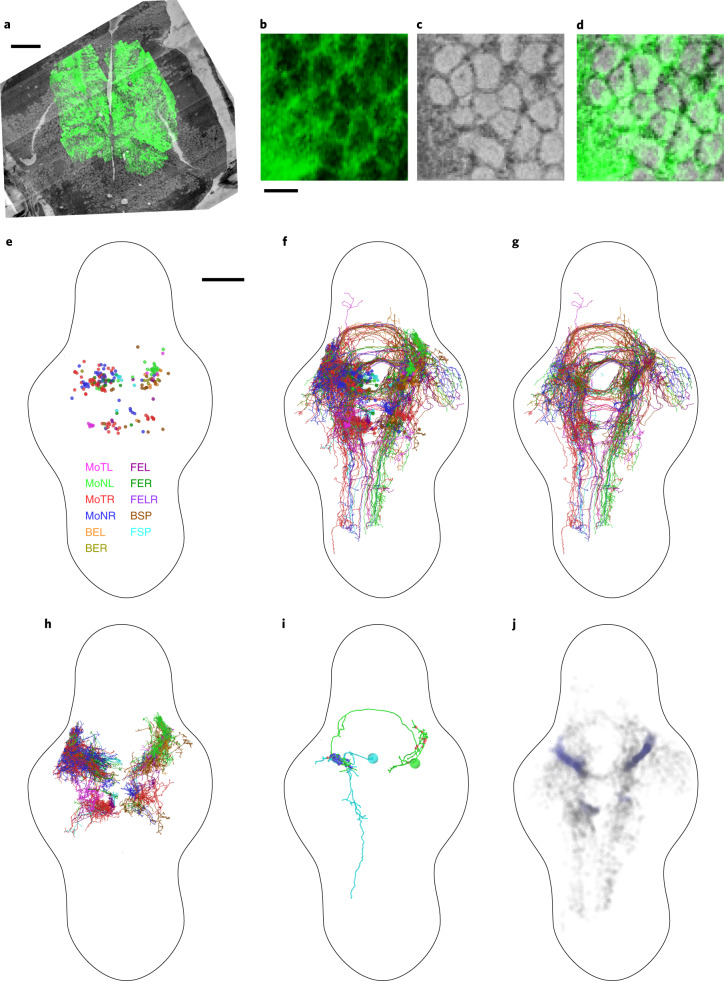
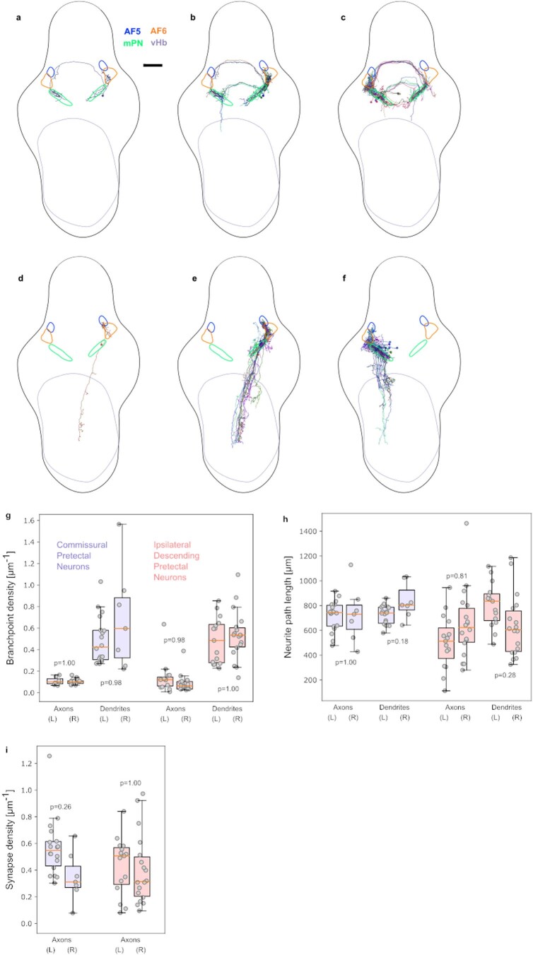
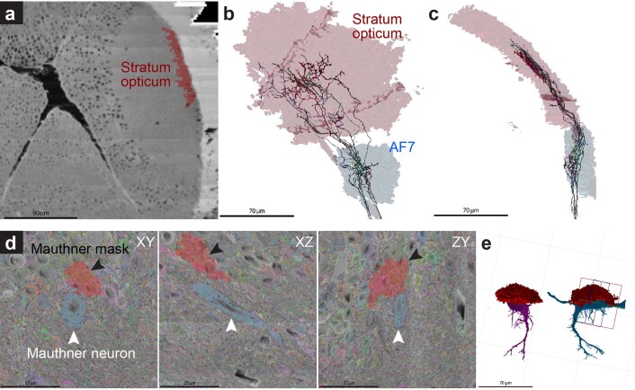
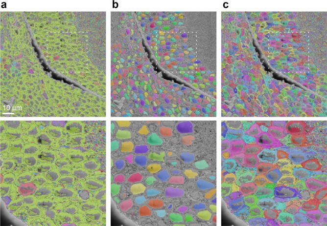
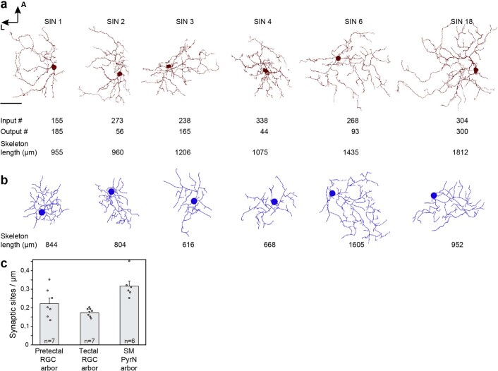
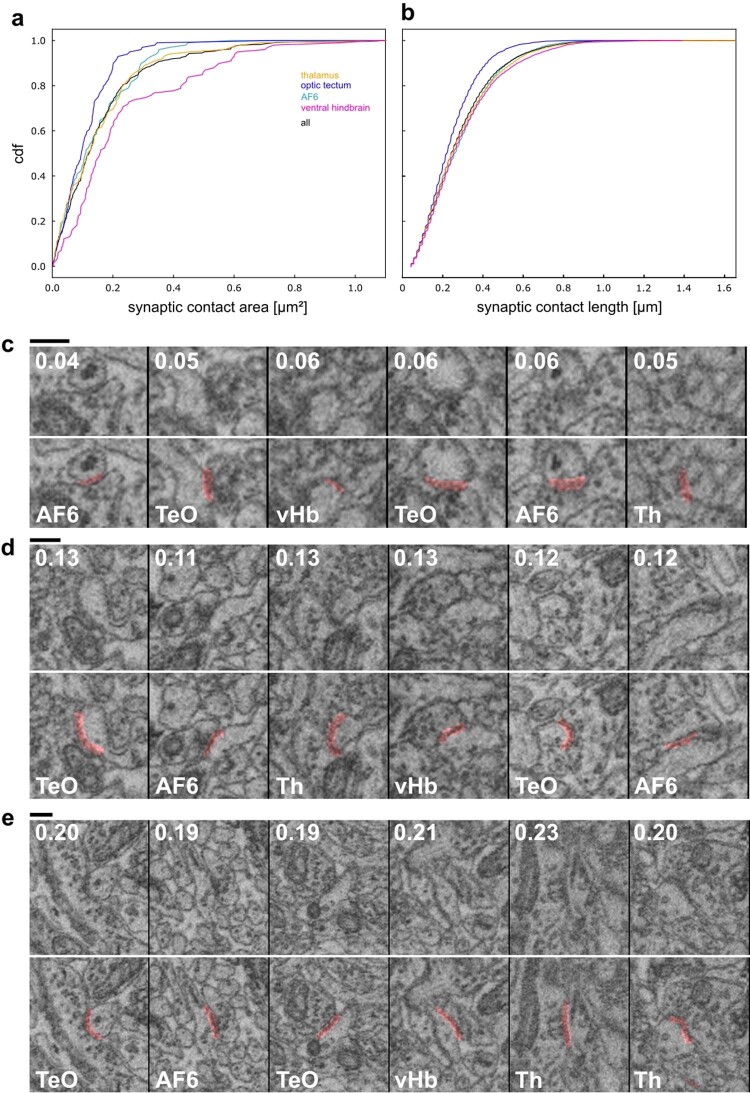
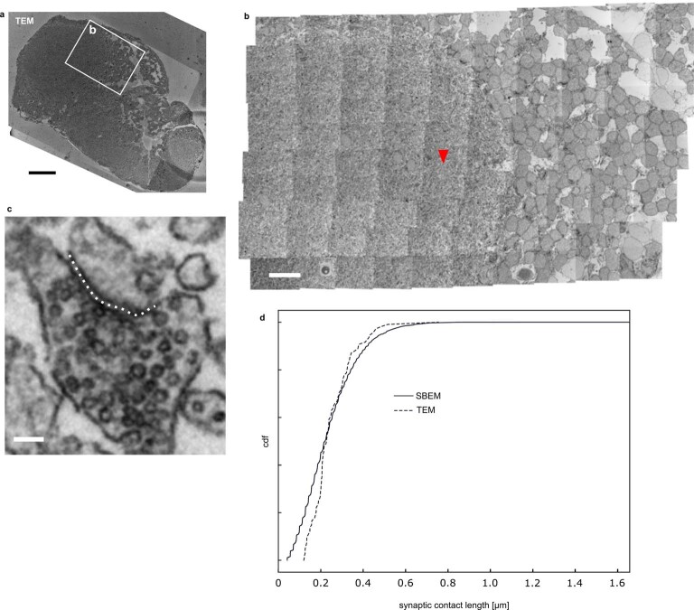
Dense reconstruction of synaptic connectivity requires high-resolution electron microscopy images of entire brains and tools to efficiently trace neuronal wires across the volume. To generate such a resource, we sectioned and imaged a larval zebrafish brain by serial block-face electron microscopy at a voxel size of 14 × 14 × 25 nm³. We segmented the resulting dataset with the flood-filling network algorithm, automated the detection of chemical synapses and validated the results by comparisons to transmission electron microscopic images and light-microscopic reconstructions. Neurons and their connections are stored in the form of a queryable and expandable digital address book. We reconstructed a network of 208 neurons involved in visual motion processing, most of them located in the pretectum, which had been functionally characterized in the same specimen by two-photon calcium imaging. Moreover, we mapped all 407 presynaptic and postsynaptic partners of two superficial interneurons in the tectum. The resource developed here serves as a foundation for synaptic-resolution circuit analyses in the zebrafish nervous system.

Fig. 1. Pretectal 2P calcium imaging and whole-brain larval SBEM dataset acquisition.

a, Illustrative larval zebrafish head at 5 dpf, brain highlighted in red. b, Wire-frame representation of a 5 dpf zebrafish brain, slice stack represents location of the 2P calcium imaged volume centered on the pretectum. c,d, X-ray image (c) of sample used to calculate horizontally stacked tile pattern (d), shown here overlaid on a low-resolution vEM overview image. e, High-resolution vEM imaged brain slice stitched from individual tiles shown in d. f, The resulting high-resolution volume. g, Synaptic contact in pretectum, as highlighted in e. Scale bars, 50 μm (d–f), 500 nm (g).

Fig. 2. Mapping and EM-based reconstruction of functionally characterized pretectal neurons.

a, Single plane of GCaMP5G fluorescence registered to SBEM dataset. b–d, Zoomed view of data in a, showing GCaMP5G (b) and scanning EM image (c) individually and as overlay (d). e–i, Panels show tracings seeded from soma centers (n = 208) (e), with functional response types classified and named as in ref. , neurons skeletonized from those seeds (f), axons (g), dendrites (h) and two individual example neurons (i), for all of the functionally characterized, EM-reconstructed cells, colored by functional response type. Blue and red spheres in i indicate incoming and outgoing synapse locations, respectively. j, All synapse locations with traced (blue) and untraced (black) postsynaptic partners. MoNL, MoNR, MoTL and MoTR refer to monocular nasalward (N) or temporalward (T), left eye (L) or right eye (R). FEL, FER, BEL, BER refers to forward- (F) or backward- (B) selective, excited by left (L) or right (R) eye. FELR refers to forward-selective, excited by left and right eye. FSP and BSP refer to forward (F) or backward (B) specific. Scale bars, 50 μm (a), 5 μm (b–d) and 100 μm (e–j).

Fig. 3. Registration of LM atlas dataset and vEM stack.

a, elavl3:lynTag-RFP (red) and elavl3:H2B-GCaMP6s (false-colored in blue) fluorescence stacks, registered into a common coordinate system. Dorsal view. b, Soma (blue) and neuropil (red) prediction on low-resolution overview vEM data used as registration target, overlaid over raw data. c. Overlay of elavl3:H2B-GCaMP6s (blue) and pou4f3:mGFP (yellow) registered into the vEM brain coordinate system and shown over full resolution vEM data. Scale bars, 100 μm.

Fig. 4. Automated neurite segmentation.

a, Dorsal view of the vEM dataset with a multicolored overlay of the base segmentation. b, Close-up examples (one out of at least ten) of the segmentation in, from top left to bottom right, the tectal neuropil (highlighted in a), rostral hypothalamus, intermediate and inferior ventral medulla oblongata. c, Examples of semiautomatically reconstructed neurons. Numbers of corrected merge and split errors are given in parentheses. From left to right: dorsal thalamic projection neuron (mergers, 1; splits, 62), tectal PVIN (1, 124), inferior raphe neuron (14, 52), inferior dorsal medulla oblongata neuron (0, 23) and pretectal interneuron (0, 8). Different colors indicate neuron fragments merged manually. Scale bars, 50 µm (a), 2 µm (b) and 10 µm (c).

Fig. 5. Reconstruction of a SIN and its partners.

a, Dorsal view of the selected SIN1. Input (blue) and output (green) synapses are indicated. b, Annotated (upper panel) and raw data (lower panel) for closely neighboring input (blue) and output (green arrowhead) synapses on a SIN’s neurite (red). Arrow in a indicates synapse location. c, Dorsal view of left tectum showing cell body locations of all input (purple) and output (cyan) neurons in the anterior tectum. d, Frontal view showing the SIN (red) and its presynaptic partners (Supplementary Video 1). Arrowheads indicate RGC input synapses onto SIN cell body. Surface of tectal hemisphere is shown in gray. e, Dorsal view of SIN (red) and its input RGC axons in the SFGS layer. Close-ups on the right show that SIN neurites (arrowheads) closely follow the network of RGC axon bundles. f, The SIN (red) and its postsynaptic partners (PVINs not shown for clarity, see Supplementary Video 2 for all postsynaptic cells). The second SIN2 for which we mapped all partners is marked by an arrow. g, Dorsal view showing a network of interconnected SINs. h, Wiring diagram for proofread SINs. Colors match cells shown in g (SINs 7–11 are not visualized for clarity). Synapse numbers are indicated next to arrowheads. Scale bars, 35 µm (a), 1 µm (b) and 85 µm (c). A: anterior, L: lateral, D: dorsal.

Fig. 6. Automatic detection of synaptic contacts.

a, Dorsal view of the vEM dataset, vesicle clouds labeled in blue. b, Close-up examples of automatically segmented vesicle clouds (blue) and synaptic clefts (magenta) in thalamus (Th), pretectum (preT), optic tectum (TeO) and ventral hindbrain (vHb). c. Outline of RGC AFs 4 (left) and 7 (right). d, Volume fraction occupied by vesicle clouds, calculated for all AFs as a percentage of total area volume. Visualization adapted from mapzebrain atlas. Scale bars, 50 µm (a), 500 nm (b) and 10 µm (c).

Extended Data Fig. 1. Neurite diameter distribution.

Neurite diameter distribution for pretectal cells (cumulative density function, cdf), measured perpendicular to the main neurite axis in axons and dendrites, at 200 randomly sampled locations in each.

Extended Data Fig. 2. Between-hemisphere comparison of reconstructed pretectal cell morphology.

Fraction of skeleton branch points, taken over all cells, present in different anatomical areas for dendrites of simple (MoNL, MoNR, MoTL and MoTR) and complex (FEL, FER, BEL, BER, FELR, FSP and BSP) cells (complex left: 38, right: 36; simple left: 94, right: 40) in the left (L) and right (R) hemisphere separately (a) and in both hemispheres (b). c-d. Like a-b, for the axons. AF5, AF6: Retinal arborization fields 5 and 6, TeO: optic tectum, mPN: medial pretectal neuropil, nMLF: neuropil of the nucleus of the medial longitudinal fasciculus, vHb: ventral hindbrain neuropil. (i) and (c) indicate ipsilateral and contralateral, respectively. AF and nMLF annotations are based on LM atlas masks registered to the EM data.

Extended Data Fig. 3. Bilaterally symmetric reconstructions of two morphologically defined pretectal cell types.

Individual example of a commissural pretectal interneuron (a) and all neurons of this type with somata on the right (b) and left (c) side of the brain. d-f. Like a-c, for ipsilateral descending pretectal projection neurons. g-i. Branchpoint densities (g), neurite path lengths (h) and axonal synapse densities (i) for commissural pretectal interneurons (blue, n = 18 and 7 cells on the left and right side, respectively) and ipsilateral descending pretectal projection neurons (red, n = 15 and 18 cells on the left and right side, respectively), plotted separately for axons and dendrites and for the two brain hemispheres. AF5, AF6: Retinal arborization fields 5 and 6, mPN: medial pretectal neuropil region, vHb: ventral hindbrain neuropil. AF annotations are based on LM atlas masks registered to the EM data. Box plot center lines represent medians, box limits upper and lower quartiles, whiskers 1.5x the interquartile range. Scale bar: 100 μm.

Extended Data Fig. 4. LM-to-EM registration match precision.

Examples for the accuracy of registrations. a-c: Retinal ganglion cell axons (n = 7), which have been traced in the EM dataset and which project both to the tectal stratum opticum (SO) and the arborization field 7 (AF7), localize exclusively inside the registered mapzebrain regions. d-e: The registered mask for the Mauthner neurons, which was generated in the mapzebrain atlas (red, black arrowheads), deviates by ~20 µm from the location of the Mauthner cells in the EM dataset (blue, white arrowheads). Second Mauthner cell is shown in magenta in e.

Extended Data Fig. 5. Splitting of merged somata with nuclei segmentation.

a. Initial segmentation with prolific soma-soma mergers, b. Nucleus segmentation, c. Initial segmentation split with nucleus segmentation in (b).

Extended Data Fig. 6. Synapse density and neurite path length comparisons between LM and EM.

a-b. Comparison of reconstructed SINs from our EM dataset (a) and from our LM mapzebrain atlas (b). The number of input and output synapses is shown below each cell in (a) and the neurite path length in µm in (a) and (b). Scale bar: 30 µm. c. Quantification of synapse densities for presynaptic sites of RGCs in the pretectal AF8 and tectal AF10, and for postsynaptic sites of tectal pyramidal neurons (PyrN) in the stratum marginale (SM). Number of cells (n) is provided in each bar. Error bars are SEM.

Extended Data Fig. 7. Size of synaptic contacts.

a. Distribution of synaptic contact areas in different brain areas (n = 100 in each area). b. For the same synaptic contacts as in a, distribution of contact lengths as exposed in each intersecting slice. c. Examples of small synaptic contacts (20th to 30th percentile by area). Contact area in μm² indicated at the top, brain area at the bottom. d, e. Like c, for intermediate (45th to 55th percentile) and large (70th to 80th percentile) synapses, respectively. Scale bars: 250 nm. AF6: Retinal arborization field 6, TeO: optic tectum, vHb: ventral hindbrain, Th: thalamus.

Extended Data Fig. 8. Comparison of synaptic contact lengths in TEM image of optic tectum.

a. Overview of 35 nm section of a 5 dpf larval zebrafish prepared identically to the sample used for SBEM. b. Close-up tile mosaic in optic tectum neuropil. Arrowhead points at synapse in (c). c. Example synapse. Dotted line illustrates synaptic contact length measurement. d. Distribution of contact lengths (n = 100, randomly sampled) in this TEM image (dotted line) compared to the distribution obtained from the optic tectum in the SBEM dataset (as in Extended Data Fig. 7b). Scale bars: a. 50 μm, b. 10 μm, c. 100 nm.

Extended Data Fig. 9. Custom sample holder for reproducible larval zebrafish positioning.

a. Aluminum stub for fish embedding, b. Carbon black epoxy, including fish, cast on the sample holder, c. Schematic cross-section.

Extended Data Fig. 10. Simulation of proofreading server performance under different concurrent user loads.

a. Response time to request of meshes for cells (either complete or currently undergoing proofreading) and (b) to the request of agglomeration graph connected component containing a given supervoxel, depending on the number of concurrently active simulated users. Box plot center lines represent medians, box limits upper and lower quartiles, whiskers 1.5x the interquartile range.

References

1. White JG, Southgate E, Thomson JN, Brenner S. The structure of the nervous system of the nematode Caenorhabditis elegans. Philos. Trans. R. Soc. Lond. B Biol. Sci. 1986;314:1–340. - PubMed
1. Bargmann CI, Marder E. From the connectome to brain function. Nat. Methods. 2013;10:483–490. - PubMed
1. Ohyama T, et al. A multilevel multimodal circuit enhances action selection in Drosophila. Nature. 2015;520:633–639. - PubMed
1. Scheffer LK, et al. A connectome and analysis of the adult Drosophila central brain. eLife. 2020;9:e57443. - PMC - PubMed
1. Zheng Z, et al. A complete electron microscopy volume of the brain of adult Drosophila melanogaster. Cell. 2018;174:730–743.e22. - PMC - PubMed
Publication types
LinkOut - more resources