GUBS: Graph-Based Unsupervised Brain Segmentation in MRI Images

Abstract

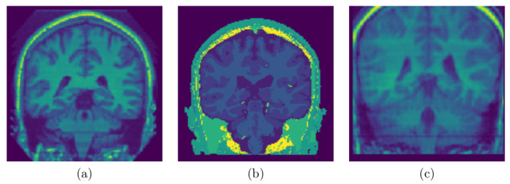
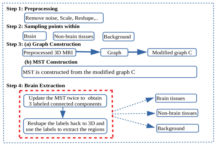
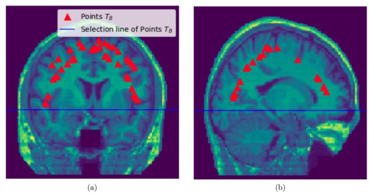
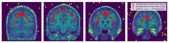
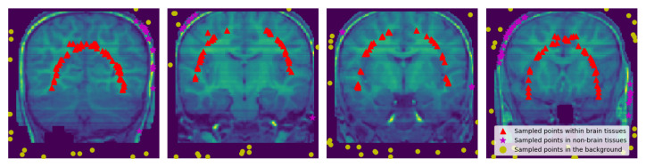
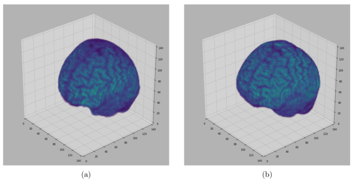
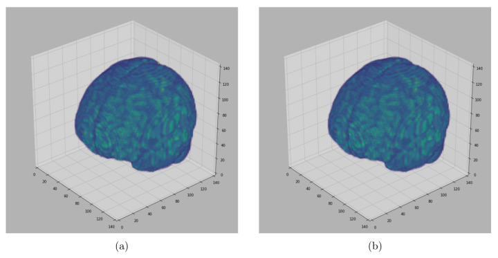
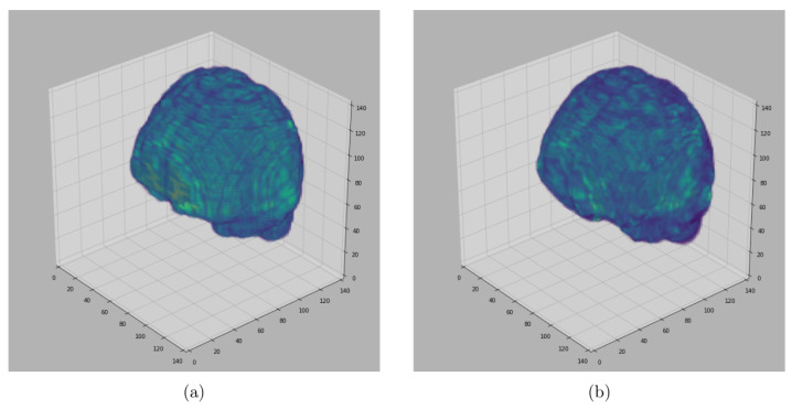
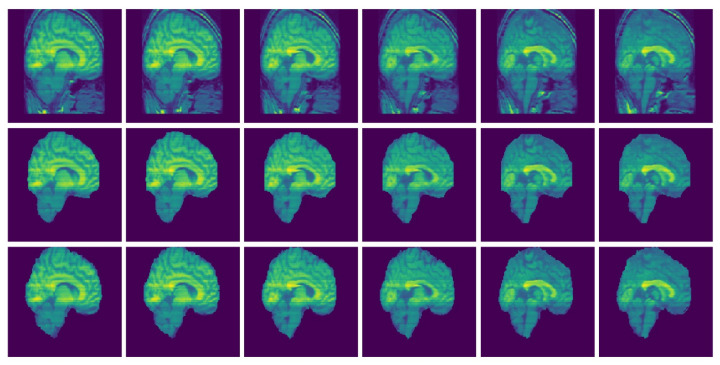
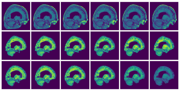
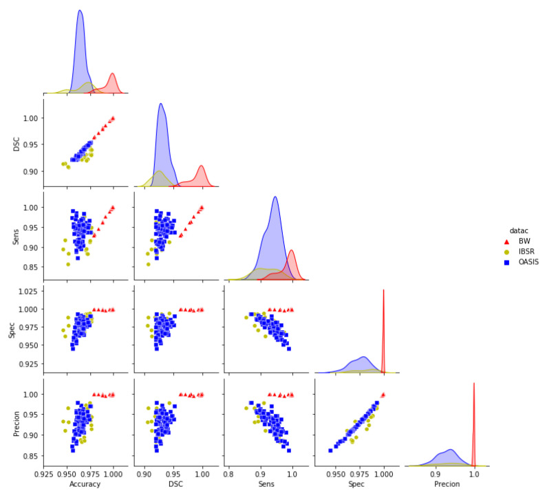
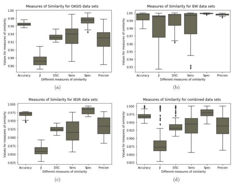
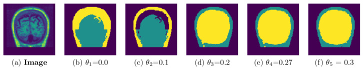
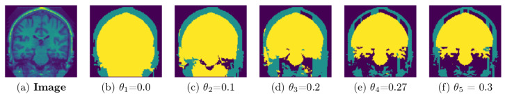
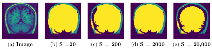
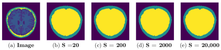
Brain segmentation in magnetic resonance imaging (MRI) images is the process of isolating the brain from non-brain tissues to simplify the further analysis, such as detecting pathology or calculating volumes. This paper proposes a Graph-based Unsupervised Brain Segmentation (GUBS) that processes 3D MRI images and segments them into brain, non-brain tissues, and backgrounds. GUBS first constructs an adjacency graph from a preprocessed MRI image, weights it by the difference between voxel intensities, and computes its minimum spanning tree (MST). It then uses domain knowledge about the different regions of MRIs to sample representative points from the brain, non-brain, and background regions of the MRI image. The adjacency graph nodes corresponding to sampled points in each region are identified and used as the terminal nodes for paths connecting the regions in the MST. GUBS then computes a subgraph of the MST by first removing the longest edge of the path connecting the terminal nodes in the brain and other regions, followed by removing the longest edge of the path connecting non-brain and background regions. This process results in three labeled, connected components, whose labels are used to segment the brain, non-brain tissues, and the background. GUBS was tested by segmenting 3D T1 weighted MRI images from three publicly available data sets. GUBS shows comparable results to the state-of-the-art methods in terms of performance. However, many competing methods rely on having labeled data available for training. Labeling is a time-intensive and costly process, and a big advantage of GUBS is that it does not require labels.

Keywords: brain tissues; minimum spanning tree; non-brain tissues; segmentation.

Figure 1

Sampled Slices: (a) Sampled slice coronal section from a 3D MRI volume OASIS data set, (b) Sampled slice coronal section from a 3D MRI volume BW data set, (c) Sampled slice coronal section from a 3D MRI volume IBSR data set. Notice the differences and the quality of data sets.

Figure 2

Schematic diagram: Flow diagram showing the steps for brain extraction. Step 1: Pre-processing to remove noise, scale values in the range of 0 and 1 and reshape the 3D magnetic resonance imaging (MRI) volume. Step 2: Sampling points within the brain, non-brain tissues, and the background. Step 3: An adjacency graph weighted by absolute intensity differences is constructed from the preprocessed 3D MRI volume. Then, nodes in the adjacency graph corresponding to the sampled points in step 2 are collapsed in their respective regions to form a graph C. From the modified graph C, a minimum spanning tree is constructed. Step 4: Brain segmentation. Nodes in C representing each of the regions of interest are the terminal nodes for the paths to be disconnected to separate the regions. First, the minimum spanning tree (MST) is modified by removing the edge with highest edge weight in the path connecting the representative nodes to separate the brain and non-brain subtrees. Again the MST is modified by removing the edge with highest edge weight in the path connecting the representative nodes to separate the non-brain and background subtrees. New labels are assigned and reshaped back to the shape of the 3D MRI.

Figure 3

Sampling points $T_B$ within the brain: (a) Sampled slice coronal section showing the selection line and points sampled within the brain, (b) Sampled slice sagittal section section showing the selection line and points sampled within the brain.

Figure 4

Sampled Points: 2D visualization of the representative coronal section from MRI image of a single subject (OASIS data) showing the sampled points within the brain, within the non-brain, and in the background region. ${\delta }_1$ and ${\delta }_2$ values were set to 15 and 3, respectively.

Figure 5

Sampled Points: 2D visualization of the representative coronal section from MRI image of a single subject (IBSR data) showing the sampled points within the brain region, within non-brain tissues, and in the background. ${\delta }_1$ and ${\delta }_2$ values were set to 15 and 3, respectively. Notice the removed part of the skull and the brain from some slices.

Figure 6

Segmented Brain (OASIS data): One representative subject representing (a) 3D brain segmented using GUBS approach (predicted), (b) 3D brain (ground truth). The masks were segmented using a custom method based on registration to an atlas, and then revised by human experts.

Figure 7

Segmented Brain (BW data): One representative subject representing (a) 3D brain segmented using GUBS approach (predicted), (b) 3D brain (ground truth). The ground truth was obtained from the labels representing cerebrospinal fluid (CSF), gray matter (GM), and white matter (WM).

Figure 8

Segmented Brain (IBSR data): One representative subject representing (a) 3D brain segmented using GUBS approach (predicted), (b) 3D brain (ground truth). The ground truth was obtained by manual-guided expert segmentation.

Figure 9

Selected MRI slices (IBSR data set): Sagittal MRI plane segmented brain. Row one: Input images, Row two: Predicted brain and Row three: Ground truth brain.

Figure 10

Selected MRI slices (OASIS data set): Sagittal MRI plane segmented brain. Row one: Input images, Row two: Predicted brain and Row three: Ground truth brain.

Figure 11

Pair plots for the measures of similarity (Combined data sets): Pair plots showing the pairwise relationship between different measures of similarity for the results obtained using GUBS across the combined data sets. DSC = Dice Similarity coefficients, Sens = Sensitivity, Spec = Specificity.

Figure 12

Boxplot for the measures of similarity (Combined Data sets): Boxplot showing variability for the measures of similarity for the results obtained using GUBS method across the combined data sets. JI = Jaccard Indices, DSC = Dice Similarity coefficients, Sens = Sensitivity, Spec = Specificity.

Figure 13

A representative coronal section from 3D MRI showing the separation of components for different thresholds: MRI from a single subject (IBSR data set) experimented using different thresholds and nodes sample size is 20,000. GUBS is run on 3D and for visualization we take 2D at the same location for all experiments.

Figure 14

A representative coronal section from 3D MRI showing the separation of components for different thresholds: MRI from a single subject (OASIS data set) experimented using different thresholds and the nodes sample size is 20,000. GUBS is run on 3D and for visualization we take 2D at the same location for all experiments.

Figure 15

A representative coronal section from 3D MRI showing the separation of components for different sample size: MRI from a single subject (IBSR data set) experimented using threshold $T=0.27$ and different size of the sampled nodes. GUBS is run on 3D and for visualization we take 2D at the same location for all experiments.

Figure 16

A representative axial section from 3D MRI showing the separation of components for different sample size: MRI from a single subject (BW data set) experimented without threshold, different size of the sampled nodes. GUBS is run on 3D and for visualization we take 2D at the same location for all experiments.

References

1. Despotović I., Goossens B., Philips W. MRI segmentation of the human brain: Challenges, methods, and applications. Comput. Math. Methods Med. 2015;2015:450341. doi: 10.1155/2015/450341. - DOI - PMC - PubMed
1. Kalavathi P., Prasath V. Methods on skull stripping of MRI head scan images—A review. J. Digit. Imaging. 2016;29:365–379. doi: 10.1007/s10278-015-9847-8. - DOI - PMC - PubMed
1. Ramon C., Garguilo P., Fridgeirsson E.A., Haueisen J. Changes in scalp potentials and spatial smoothing effects of inclusion of dura layer in human head models for EEG simulations. Front. Neuroeng. 2014;7:32. doi: 10.3389/fneng.2014.00032. - DOI - PMC - PubMed
1. Fatima A., Shahid A.R., Raza B., Madni T.M., Janjua U.I. State-of-the-art traditional to the machine-and deep-learning-based skull stripping techniques, models, and algorithms. J. Digit. Imaging. 2020;33:1443–1464. doi: 10.1007/s10278-020-00367-5. - DOI - PMC - PubMed
1. Li J., Erdt M., Janoos F., Chang T.C., Egger J. Computer-Aided Oral and Maxillofacial Surgery. Academic Press; Cambridge, MA, USA: 2021. Medical image segmentation in oral-maxillofacial surgery; pp. 1–27.