Descending neuron population dynamics during odor-evoked and spontaneous limb-dependent behaviors

Abstract

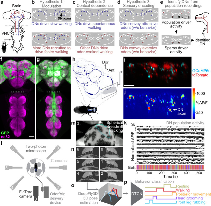
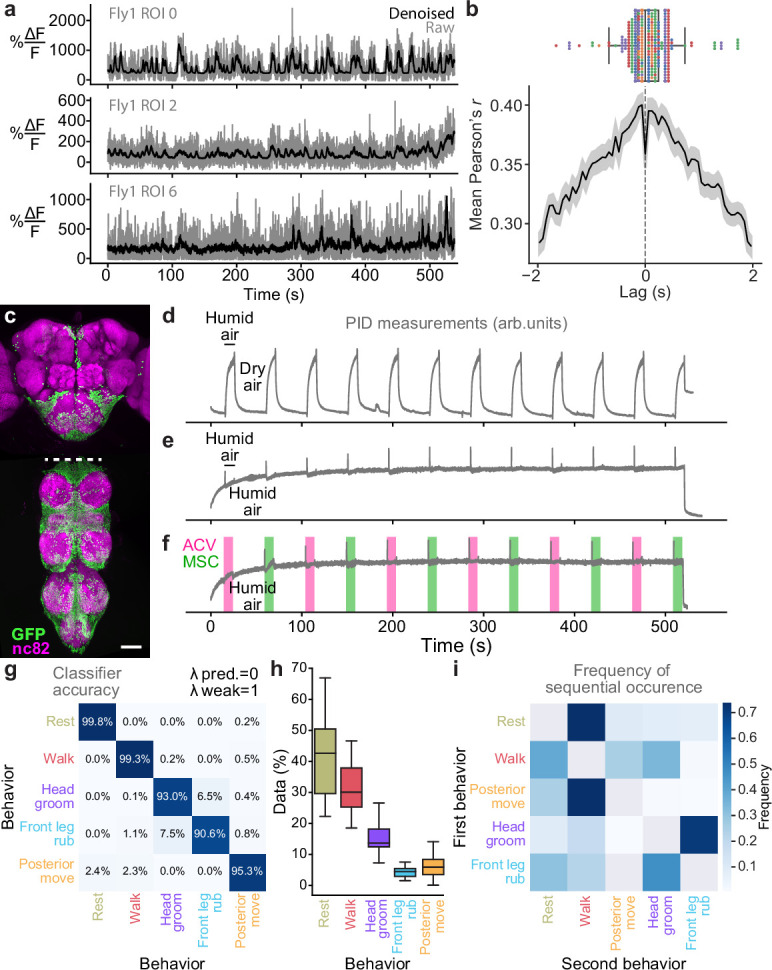
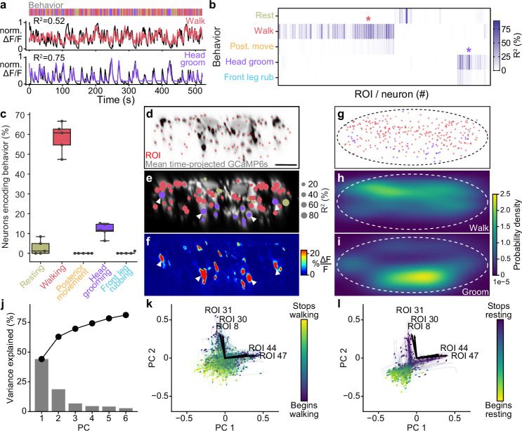
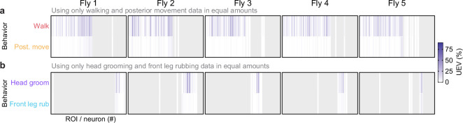
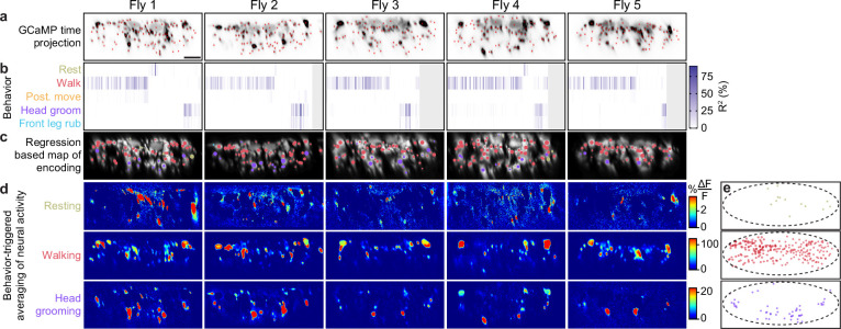
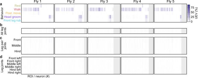
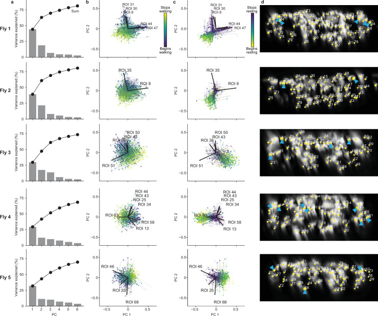
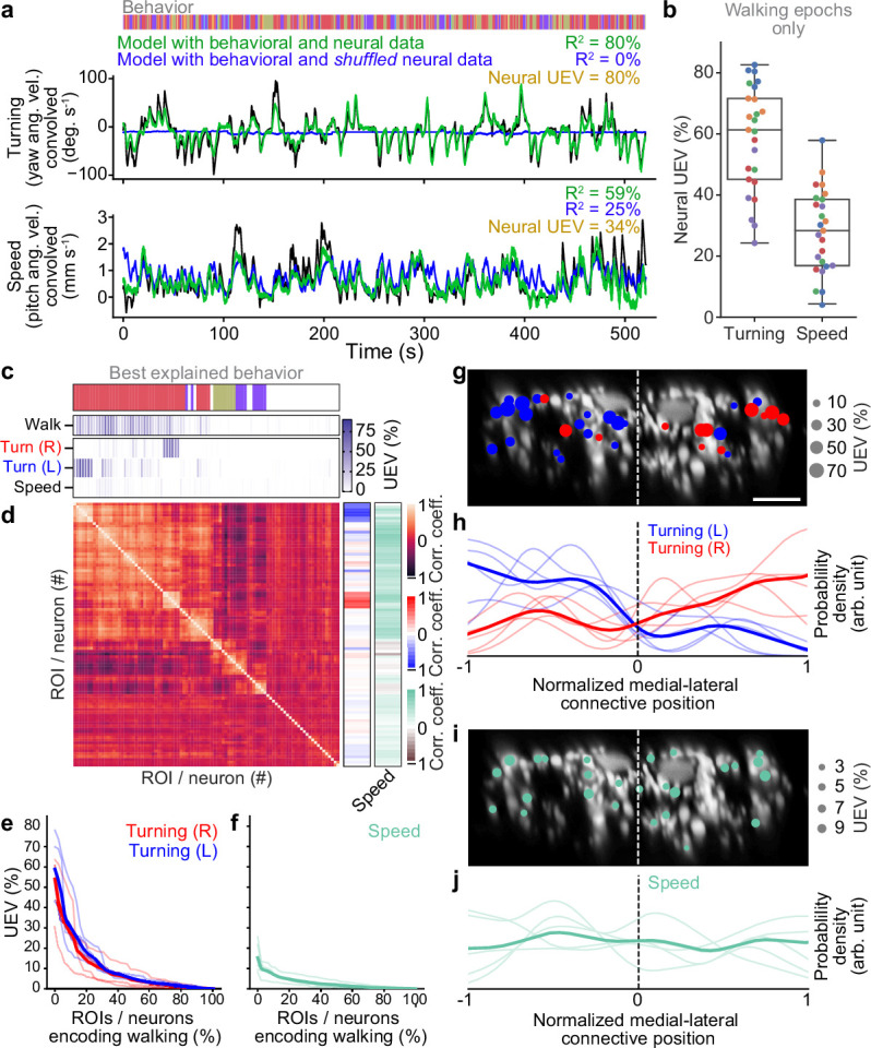
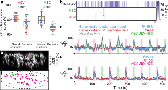
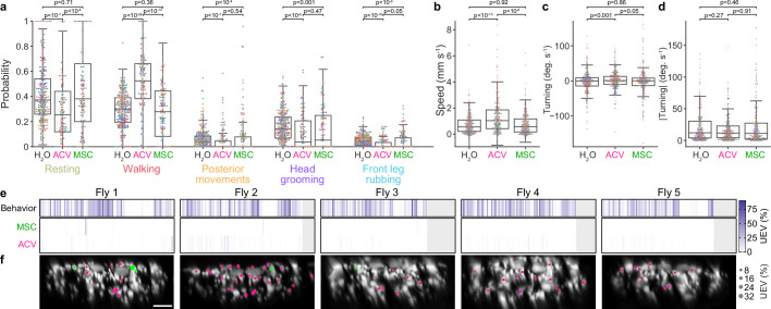
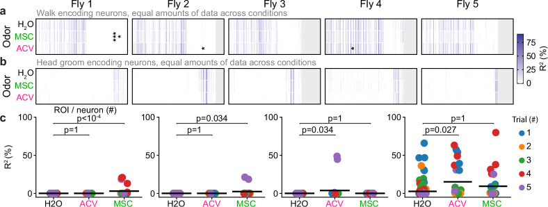
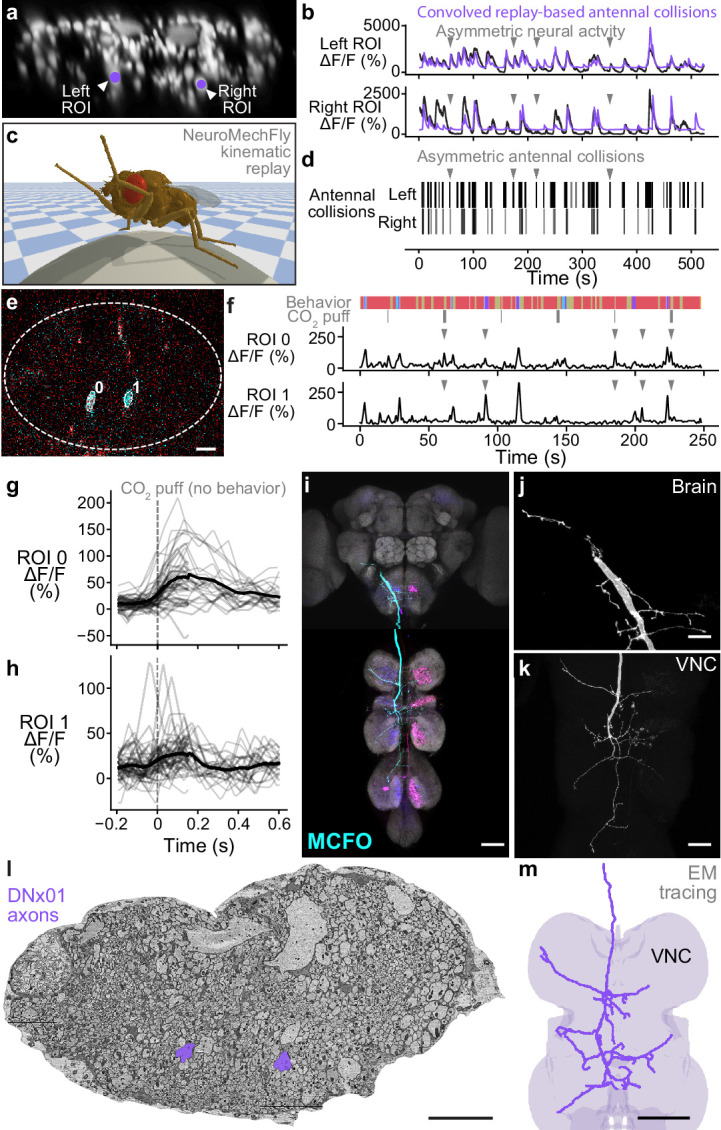
Deciphering how the brain regulates motor circuits to control complex behaviors is an important, long-standing challenge in neuroscience. In the fly, Drosophila melanogaster, this is coordinated by a population of ~ 1100 descending neurons (DNs). Activating only a few DNs is known to be sufficient to drive complex behaviors like walking and grooming. However, what additional role the larger population of DNs plays during natural behaviors remains largely unknown. For example, they may modulate core behavioral commands or comprise parallel pathways that are engaged depending on sensory context. We evaluated these possibilities by recording populations of nearly 100 DNs in individual tethered flies while they generated limb-dependent behaviors, including walking and grooming. We found that the largest fraction of recorded DNs encode walking while fewer are active during head grooming and resting. A large fraction of walk-encoding DNs encode turning and far fewer weakly encode speed. Although odor context does not determine which behavior-encoding DNs are recruited, a few DNs encode odors rather than behaviors. Lastly, we illustrate how one can identify individual neurons from DN population recordings by using their spatial, functional, and morphological properties. These results set the stage for a comprehensive, population-level understanding of how the brain's descending signals regulate complex motor actions.

Keywords: D. melanogaster; descending neuron; grooming; limb; neuroscience; population imaging; two-photon microscopy; walking.

Figure 1.. Recording descending neuron (DN) population activity and animal behavior.

(a) Schematic of the Drosophila nervous system showing DNs projecting from the brain to motor circuits in the ventral nerve cord (VNC). For clarity, only two pairs of DNs (red and blue) are shown. Indicated (dashed gray line) is the coronal imaging region-of-interest (ROI) in the thoracic cervical connective. (b) In a ‘modulation’ framework for DN population control, new DNs (red) may be recruited to modulate ongoing behaviors primarily driven by core DNs (blue). Each ellipse is an individual DN axon (white, blue, and red). (c) In a ‘context dependence’ framework for DN population control, different DNs may be recruited to drive identical behaviors depending on sensory context. (d) Alternatively, in a ‘sensory encoding’ framework, many DNs may not drive or be active during behaviors but rather transmit raw sensory signals to the VNC. (e) An approach for deriving DN cell identity from population recordings. One may first identify sparse transgenic strains labeling specific neurons from DN populations (circled in black) using their functional attributes/encoding, positions within the cervical connective, and the shapes of their axons. Ultimately, one can use sparse morphological data to find corresponding neurons in the brain and VNC connectomes. (f, g) Template-registered confocal volume z-projections illustrating a ‘brain only’ driver line (otd-nls:FLPo; R57C10-GAL4,tub>GAL80>) expressing (f) a nuclear (histone-sfGFP) or (g) a cytosolic (smGFP) fluorescent reporter. Scale bar is 50 μm. Location of two-photon imaging plane in the thoracic cervical connective is indicated (white dashed lines). Tissues are stained for GFP (green) and neuropil (‘nc82’, magenta). (h) Schematic of the VNC illustrating the coronal (x–z) imaging plane. Dorsal-ventral (‘Dor’) and anterior–posterior (‘Ant’) axes are indicated. (i) Denoised two-photon image of DN axons passing through the thoracic cervical connective. Scale bar is 10 μm. (j) Two-photon imaging data from panel (i) following motion correction and $\%\mathrm{\Delta }F/F$ color-coding. An ROI (putative DN axon or closely intermingled axons) is indicated (white dashed circle). (k) Sample normalized $\%\mathrm{\Delta }F/F$ time-series traces for 28 (out of 95 total) ROIs recorded from one animal. Behavioral classification at each time point is indicated below and is color-coded as in panel (p). (l) Schematic of system for recording behavior and delivering odors during two-photon imaging (not to scale) while a tethered fly walks on a spherical treadmill. (m) Spherical treadmill ball rotations (fictive walking trajectories) are captured using the front camera and processed using FicTrac software. Overlaid (cyan) is a sample walking trajectory. (n) Video recording of a fly from six camera angles. (o) Multiview camera images are processed using DeepFly3D to calculate 2D poses and then triangulated 3D poses. These 3D poses are further processed to obtain joint angles. (p) Joint angles are input to a dilated temporal convolutional network (DTCN) to classify behaviors including walking, resting, head (eye and antennal) grooming, front leg rubbing, or posterior (abdominal and hindleg) movements.

Figure 1—figure supplement 1.. Supporting details regarding neural denoising, driver line expression, odor stimulation, and behavior quantification.

(a) Example $\mathrm{\Delta }F/F$ traces extracted from optic-flow registered ‘Raw’ (gray) and corresponding ‘Denoised’ (black) images. (b, top) Time lag between denoised and raw $\mathrm{\Delta }F/F$ traces with maximal cross-correlation. Overlaid are individual data points from each fly (color-coded). (b, bottom) Average cross-correlation for all regions-of-interest (ROIs) and flies (solid line) and corresponding 95% confidence interval (shaded region). (c) Z-projected confocal image of the genetic complement of the ‘brain only’ driver line (otd-nls:FLPo,tub>stop>GAL80; R57C10-GAL4) expressing nuclear GFP. Shown are staining for neuropil (‘nc82’, magenta) and GFP (green). Scale bar is 50 μm. (d–f) Photoionization detector (PID) measurements during odor delivery switching between (d) humid and dry air, (e) humid and humid air (to measure valve-related transients) or (f) humid air, methyl salicylate (MSC), and apple cider vinegar (ACV) odors. (g) Results of leave-one-fly-out cross-validation hyperparameter search for the behavior classifier. The values ${\lambda }_{weak}=1$ and ${\lambda }_{pred}=0$ yield the highest classification accuracy. (h) Relative frequency of classified behaviors in our dataset (n = 5 animals). (i) The frequency of transitions between sequential behaviors.

Figure 1—figure supplement 2.. The range of joint angles explored during fly behaviors.

Each subplot shows the normalized kernel density estimate of the distribution of a specific angle for the front, middle, or hind legs. Joint angles from all time points and flies were pooled to generate kernel density estimates. The angles are defined as described in Lobato-Rios et al., 2022.

Figure 2.. Encoding of behavior in descending neuron (DN) populations.

(a) Shown for walking (top) and head grooming (bottom) are the activity (normalized and cross-validation predicted $\mathrm{\Delta }F/F$) of individual walk- and head groom-encoding DNs (red and purple lines), as well as predicted $\mathrm{\Delta }F/F$ traces derived by convolving binary behavior regressors with a calcium response function (crf) (black lines). The output of the behavior classifier is shown (color bar). (b) The cross-validation mean of behavioral variance explained by each of 95 DNs from one animal. Colored asterisks are above the two DNs illustrated in panel (a). (c) The percentage of DNs encoding each classified behavior across five animals. Box plots indicate the median, lower, and upper quartiles. Whiskers signify furthest data points. (d) Mean time projection of GCaMP6s fluorescence over one 9 min recording. Image is inverted for clarity (high mean fluorescence is black). Manually identified DN regions of interest (ROIs) are shown (red rectangles). Scale bar is 10 μm. Panels (d–i) share the same scale. (e) DNs color-coded (as in panel c) by the behavior their activities best explain. Radius scales with the amount of variance explained. Prominent head groom-encoding neurons that are easily identified across animals are indicated (white arrowheads). (f) Behavior-triggered average $\mathrm{\Delta }F/F$ image for head grooming. Prominent head grooming DNs identified through linear regression in panel (e) are indicated (white arrowheads). (g) Locations of DNs color-coded by the behavior they encode best. Data are from five animals. (h, i) Kernel density estimate based on the locations of (h) walking or (i) head grooming DNs in panel (g). (j) Amount of variance explained by the principal components (PCs) of neural activity derivatives during walking. (k, l) Neural activity data during (k) walking and (l) resting evolve on two lobes. The PC embedding was trained on data taken during walking only. Colored lines indicate individual epochs of (k) walking and (l) resting. Time is color-coded and the temporal progressions of each epoch is indicated (arrowheads). Note that color scales are inverted to match the color at transitions between walking and resting. Black arrows indicate ROIs with high PC loadings. ROI number corresponds to the matrix position in panel (b). For their locations within this fly’s cervical connective, see Figure 2—figure supplement 4d.

Figure 2—figure supplement 1.. Disentangling the relative encoding of frequently sequential behavior pairs.

(a, b) Cross-validation mean of neural variance uniquely explained by (a) walking versus posterior movements or (b) head grooming versus front leg rubbing. In both cases, only data acquired during the two compared behaviors were analyzed. Additionally, data were balanced to have an equal amount across both behaviors.

Figure 2—figure supplement 2.. Encoding of behavior in descending neuron (DN) populations across individual animals.

(a) Mean time projections of GCaMP6s fluorescence over a 9 min recording for five animals. Images are inverted for clarity, illustrating high mean fluorescence (black). Manually identified DN regions of interest (ROIs) are shown (red rectangles). Scale bar is 10 μm. All subpanels and panels (c, d) share the same scale. (b) The cross-validation mean of behavioral variance explained by DNs for each animal (Fly 1: n = 95 ROIs; Fly 2: n = 86 ROIs; Fly 3: n = 75 ROIs; Fly 4: n = 81 ROIs; Fly 5: n = 79 ROIs). (c) DNs color-coded by the behavior their activities best explain. Radius scales with the amount of variance explained. (d) Behavior-triggered average $\mathrm{\Delta }F/F$ images for the most common behaviors—resting, walking, and head grooming. (e) Locations of DNs for the classified behavior they encode best. Data are pooled across five animals.

Figure 2—figure supplement 3.. Neural variance explained by distinct kinematic features.

(a–d) Amount of neural variance that can be uniquely explained by (a) classified behaviors (taken from the previous figure), (b) all joint movements, (c) leg pair movements, or (d) individual leg movements.

Figure 2—figure supplement 4.. Principal component (PC) analysis of neural activity during walking and resting across individual animals.

(a) Amount of variance explained by six PCs of neural activity derivatives during walking for five individual flies. (b, c) The derivative of neural activity during (b) walking and (c) resting. PC embeddings were trained on data taken during walking only. Colored trajectories are individual epochs of (b) walking and (c) resting. Time is color-coded and the temporal progression of each epoch is indicated (arrowheads). Note that color scales are inverted to match the color at transitions between walking and resting. Black arrows indicate PC loadings for descending neurons (DNs) with vectors longer than $\sqrt{0.1}$. Region of interest (ROI) numbers correspond to the connective image in panel (d). (d) Locations of ROIs for each individual animal (yellow circles). Numbers are based on the order in Figure 2—figure supplement 2b. Circle radii indicate the norm of the loadings for PCs 1 and 2 (i.e., the lengths of the vectors in panels b and c). ROIs with the largest loadings are indicated (cyan arrowheads).

Figure 3.. Turning and speed encoding in descending neuron (DN) populations.

(a) Predictions of (top) turning and (bottom) walking speed modeled using convolved behavior regressors and all neurons in one animal. Shown are predictions (green) with all regressors intact or (blue) with neural data shuffled across time. Indicated are $R^2$ values obtained by comparing predicted and real (black) turning and walking speed. These are subtracted to obtain neural unique explained variance (UEV). The fly’s behavior throughout the recording is indicated (color bar). (b) UEV obtained only using data taken during walking, thus accounting for trivial explanations of speed and turning variance resulting from transitions between resting and walking. Shown are data from five trials each for five flies (color-coded). (c) UEV of each DN from one animal for walking speed or left and right turning ordered by clustering of Pearson’s correlation coefficients in panel (d). Walking $R^2$ values are the same as in Figure 2b but reordered according to clustering. The models for turning and walking speed were obtained using behavior regressors as well as neural activity. To compute the UEV, activity for a given neuron was shuffled temporally. The behavior whose variance is best explained by a given neuron is indicated (color bar). (d) Pearson’s correlation coefficient matrix comparing neural activity across DNs ordered by clustering. Shown as well are the correlation of each DN’s activity with right, left, and forward walking (right). (e, f) UEV for (e) turning or (f) speed for DNs that best encode walking. Neurons are sorted by UEV. Shown are the distributions for individuals (translucent lines), and the mean across all animals (opaque line). (g) Locations of turn-encoding DNs (UEV > 5%), color-coded by preferred direction (left, blue; right, red). Circle radii scale with UEV. Dashed white line indicates the approximate midline of the cervical connective. Scale bar is 10 μm for panels (g) and (i). (h) Kernel density estimate of the distribution of turn encoding DNs. Shown are the distributions for individuals (translucent lines), and the mean distribution across all animals (opaque lines). Probability densities are normalized by the number of DNs along the connective’s medial–lateral axis. (i) Locations of speed encoding DNs (UEV > 2%). Circle radii scale with UEV. Dashed white line indicates the approximate midline of the cervical connective. (j) Kernel density estimate of the distribution of speed encoding DNs. Shown are the distributions for individuals (translucent lines) and the mean distributions across all animals (opaque lines). Probability densities are normalized by the number of DNs along the connective’s medial–lateral axis.

Figure 3—figure supplement 1.. Backward walking is infrequent and brief.

Compared to forward walking epochs, in our data we measured (a) fewer and (b) shorter backward walking epochs. (c) There was also a limited dynamic range in backward walking speed. In all panels colors indicates fly identities. In panels (b) and (c) circles indicate the values of 700 randomly selected epochs (subsampled for clarity). Box plots indicate the median, lower, and upper quartiles. Whiskers signify 1.5× the interquartile range.

Figure 3—figure supplement 2.. Turning and speed encoding in descending neuron (DN) populations across individual animals.

(a) Unique explained variance (UEV) of each DN from individual animals for left and right turning or walking speed. Walking $R^2$ values are taken from Figure 2—figure supplement 2b. The model for turning and speed was obtained using behavior regressors as well as neural activity. To compute the UEV, activity for a given neuron was temporally shuffled. The behavior whose variance is best explained by a given neuron is indicated (top). Neurons are ordered as in panel (b). (b) Pearson’s correlation coefficient matrix comparing neural activity across DNs is ordered by hierarchical clustering. Shown as well are the correlations of each DN’s activity with right, left, and forward walking (right). Neurons are ordered as in panel (a). (c) Locations of turn encoding DNs (UEV > 5%), color-coded by preferred direction (left, blue; right, red). Circle radii scale with UEV. Dashed white line indicates the approximate midline of the cervical connective. Scale bars are 10 μm for all subpanels and panel (e). (d) Kernel density estimates of the distributions of turn encoding DNs across individuals (opaque lines). Probability densities are normalized by the number of DNs along the connective’s medial–lateral axis. (e) Locations of speed encoding DNs (UEV > 2%). Circle radii scale with UEV. Dashed white line indicates the approximate midline of the cervical connective. (f) Kernel density estimates of the distributions of speed encoding DNs across individuals (opaque lines). Probability densities are normalized by the number of DNs along the connective medial–lateral axis.

Figure 4.. Odor encoding in descending neuron (DN) populations.

(a) Neural residuals—obtained by subtracting convolved behavior regressors from raw neural data—can predict the presence of an odor significantly better than behavior regressors convolved with a calcium response function (‘Behavior’). Two-sided Mann–Whitney U-test. The classification score was obtained using a linear discriminant classifier with cross-validation. Shown are five trials for five animals (color-coded). (b) Matrix showing the cross-validated ridge regression unique explained variance (UEV) of a model that contains behavior and odor regressors for one animal. The first row (‘Behavior’) shows the composite $R^2$ for all behavior regressors with odor regressors shuffled. The second and third rows show the UEVs for regressors of the odors methyl salicylate (MSC) or apple cider vinegar (ACV), respectively. Colored asterisks indicate neurons illustrated in panel (a). (c, d) Example DNs best encoding (c) MSC or (d) ACV, respectively. Overlaid are traces of neural activity (gray), row one in the matrix (blue), and row one with odor data shuffled (red). (e, f) Locations of odor encoding neurons in (e) one individual and (f) across all five animals. Scale bar is 10 μm.

Figure 4—figure supplement 1.. Odor-modulated behaviors and encoding in descending neuron (DN) populations across individuals.

(a) The probabilities that classified behaviors occur during periods of stimulation with humidified air, apple cider vinegar (ACV), or methyl salicylate (MSC) odors. P-values indicate the significance level for a two-sided Mann–Whitney U-test. (b–d) Swarm plots showing a subset of 250 randomly sampled points indicating (b) walking speed, (c) turning angular velocity, and (d) absolute value of turning angular velocity during periods of stimulation with humidified air, ACV, or MSC odors. (e) Matrices showing the cross-validated ridge regression unique explained variance (UEV) of models that contain behavior and odor regressors for five individual animals. The first row (‘Behavior’) shows the composite $R^2$ for all behavior regressors and shuffled odor regressors. The second and third rows show UEVs for the odor regressors MSC and ACV, respectively. (f) Locations of odor encoding neurons (UEV > 5%) across five individual animals. Scale bar is 10 μm and applies to all images. Color indicates odor. Radii scale with the amount of variance explained.

Figure 4—figure supplement 2.. Largely identical descending neuron (DN) populations are recruited during walking and head grooming irrespective of odor context.

(a, b) Amount of (a) walking or (b) head grooming variance explained by each DN using only frames during presentation of humidified air, apple cider vinegar (ACV), or methyl salicylate (MSC). Data during humidified air presentation were split into groups to match the amount of data available during ACV and MSC presentation. Indicated are cases where a two-sided Mann–Whitney U-test comparing the cross-validation folds between humidified air and each of the odors yielded significant differences after Bonferroni correction for multiple comparisons (*${\displaystyle \mathrm{p}<0.05}$; ***${\displaystyle \mathrm{p}<0.001}$). (c) Individual region of interest (ROI) data points resulting in significant differences across conditions by a two-sided Mann–Whitney U-test (shown from left to right: fly 1, ROI 82; fly 1, ROI 87; fly 2, ROI 74; fly 4, ROI 28). Each point is the result of a single cross-validation fold from a single trial. p-Values shown are after Bonferroni correction for multiple comparisons.

Figure 5.. Identifying a pair of antennal deflection-encoding descending neurons (DNs) from population recordings.

(a) A pair of head groom-encoding DNs (purple circles and white arrowheads) can be identified from DN population recordings based on their shapes, locations, and activity patterns. (b) Example $\mathrm{\Delta }F/F$ traces (black) of DNs highlighted in panel (a). Sample time points with bilaterally asymmetric neural activity are indicated (gray arrowheads). Overlaid is a prediction of neural activity derived by convolving left and right antennal collisions measured through kinematic replay in the NeuroMechFly physics simulation (purple). (c) Kinematic replay of recorded joint angles in NeuroMechFly allow one to infer antennal collisions from real, recorded head grooming. (d) Left and right antennal collisions during simulated replay of head grooming shown in panel (b). Sample time points with bilaterally asymmetric collisions are indicated (gray arrowheads). (e) Two-photon image of the cervical connective in a R65D11>OpGCaMP6f, tdTomato animal. Overlaid are regions of interest (ROIs) identified using AxoID. The pair of axonal ROIs are in a similar ventral location and have a similarly large relative size like those seen in DN population recordings. Scale bar is 5 μm. (f) Sample neural activity traces from ROIs 0 and 1. Bilaterally asymmetric neural activity events (gray arrowheads), behaviors (color bar), and CO₂ puffs directed at the antennae (gray bars) are indicated. (g, h) CO₂ puff-triggered average of neural activity for ROIs (g) 0 and (h) 1. Only events in which animals did not respond with head grooming or front leg rubbing were used. Stimuli were presented at $t=0$. Shown are individual responses (gray lines) and their means (black lines). (i) Confocal volume z-projection of MultiColor FlpOut (MCFO) expression in an R65D11-GAL4 animal. Cyan neuron morphology closely resembles DNx01 (Namiki et al., 2018). Scale bar is 50 μm. (j, k) Higher-magnification MCFO image, isolating the putative DNx01 from panel (i), of the (j) brain and (k) ventral nerve cord (VNC). Scale bars are 20 μm. (l) The locations of axons in the cervical connective (purple) from neurons identified as DNx01. Scale bar is 10 μm. (m) Manual reconstruction of a DNx01 from panel (l). Scale bar is 50 μm.

References

1. Ache JM, Namiki S, Lee A, Branson K, Card GM. State-dependent decoupling of sensory and motor circuits underlies behavioral flexibility in Drosophila. Nature Neuroscience. 2019a;22:1132–1139. doi: 10.1038/s41593-019-0413-4. - DOI - PMC - PubMed
1. Ache JM, Polsky J, Alghailani S, Parekh R, Breads P, Peek MY, Bock DD, von Reyn CR, Card GM. Neural basis for looming size and velocity encoding in the Drosophila giant fiber escape pathway. Current Biology. 2019b;29:1073–1081. doi: 10.1016/j.cub.2019.01.079. - DOI - PubMed
1. Aimon S, Katsuki T, Jia T, Grosenick L, Broxton M, Deisseroth K, Sejnowski TJ, Greenspan RJ. Fast near-whole-brain imaging in adult Drosophila during responses to stimuli and behavior. PLOS Biology. 2019;17:e2006732. doi: 10.1371/journal.pbio.2006732. - DOI - PMC - PubMed
1. Aimon S, Cheng KY, Gjorgjieva J, Kadow ICG. Walking Elicits Global Brain Activity in Drosophila. bioRxiv. 2022 doi: 10.1101/2022.01.17.476660. - DOI
1. Asahina K, Watanabe K, Duistermars BJ, Hoopfer E, González CR, Eyjólfsdóttir EA, Perona P, Anderson DJ. Tachykinin-expressing neurons control male-specific aggressive arousal in Drosophila. Cell. 2014;156:221–235. doi: 10.1016/j.cell.2013.11.045. - DOI - PMC - PubMed
Publication types
LinkOut - more resources