Agricultural land use shapes dispersal in white-tailed deer (Odocoileus virginianus)

Abstract

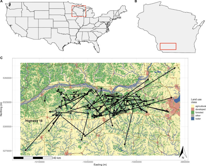
Background: Dispersal is a fundamental process to animal population dynamics and gene flow. In white-tailed deer (WTD; Odocoileus virginianus), dispersal also presents an increasingly relevant risk for the spread of infectious diseases. Across their wide range, WTD dispersal is believed to be driven by a suite of landscape and host behavioral factors, but these can vary by region, season, and sex. Our objectives were to (1) identify dispersal events in Wisconsin WTD and determine drivers of dispersal rates and distances, and (2) determine how landscape features (e.g., rivers, roads) structure deer dispersal paths.

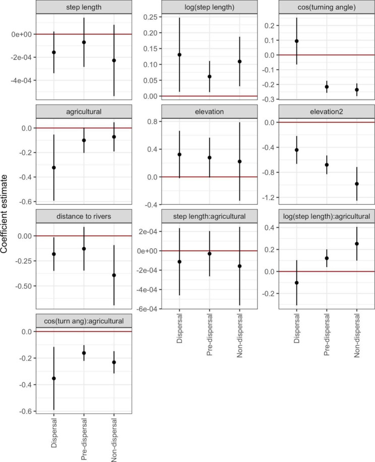
Methods: We developed an algorithmic approach to detect dispersal events from GPS collar data for 590 juvenile, yearling, and adult WTD. We used statistical models to identify host and landscape drivers of dispersal rates and distances, including the role of agricultural land use, the traversability of the landscape, and potential interactions between deer. We then performed a step selection analysis to determine how landscape features such as agricultural land use, elevation, rivers, and roads affected deer dispersal paths.

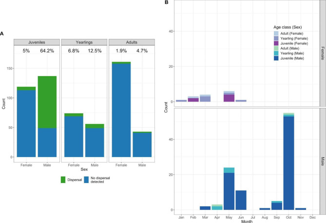
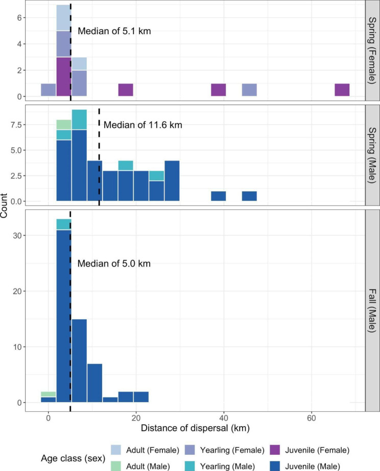
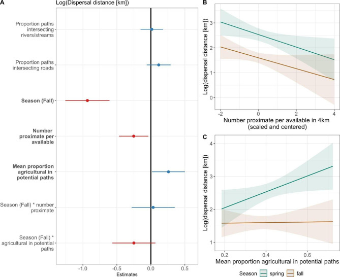
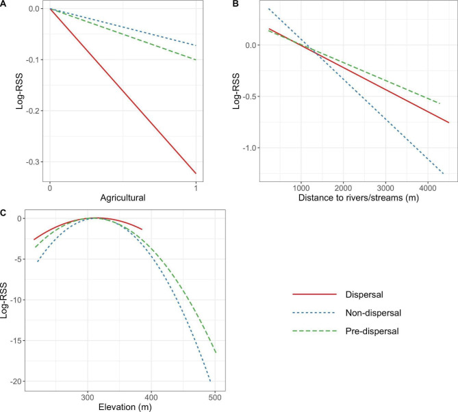
Results: Dispersal predominantly occurred in juvenile males, of which 64.2% dispersed, with dispersal events uncommon in other sex and age classes. Juvenile male dispersal probability was positively associated with the proportion of the natal range that was classified as agricultural land use, but only during the spring. Dispersal distances were typically short (median 5.77 km, range: 1.3-68.3 km), especially in the fall. Further, dispersal distances were positively associated with agricultural land use in potential dispersal paths but negatively associated with the number of proximate deer in the natal range. Lastly, we found that, during dispersal, juvenile males typically avoided agricultural land use but selected for areas near rivers and streams.

Conclusion: Land use-particularly agricultural-was a key driver of dispersal rates, distances, and paths in Wisconsin WTD. In addition, our results support the importance of deer social environments in shaping dispersal behavior. Our findings reinforce knowledge of dispersal ecology in WTD and how landscape factors-including major rivers, roads, and land-use patterns-structure host gene flow and potential pathogen transmission.

Keywords: Agricultural land use; Cervid; Chronic wasting disease; Gene flow; Movement barriers; Pathogen spread; Resource selection; Social ecology; Step selection analysis; Wisconsin.

Fig. 1

Counts of southwest Wisconsin white-tailed deer dispersal by sex and age class. In (A), dispersals are shown in green (top of bar) and percentages above each bar give the percent dispersers for each sex/age class combination. In (B), the timing of dispersals is shown by sex (females in upper panel, males in lower) and age class (color or shading of bars). Note that in (B), individuals that dispersed two times are shown twice to show the full distribution of dispersal events, and the y-axes are identical to facilitate visual comparison by sex

Fig. 2

Histograms of Wisconsin white-tailed deer dispersal distances (in km), stratified by season and sex. Bars are colored by the age class of individuals at dispersal. Females only dispersed in the spring, and are shown in the top panel; male dispersal distances in the spring and fall are shown in the middle and bottom panels, respectively. Y-axes vary between panels, with the bottom panel the largest due to its higher count values. Median dispersal distances per season and sex are shown with vertical dashed lines. Note that individuals that dispersed two times (n = 6) are shown twice to show the full distribution of dispersal distances

Fig. 3

Maps showing (A) the study area locale of Wisconsin (red dashed box) in the context of the United States, (B) the study area and surrounding land (red solid box) in the context of Wisconsin, and (C) white-tailed deer dispersal events with the landscape colored by land use class. In (B), the solid red box corresponds to the bounds of the area shown in (C). The arrows in (C) initiate at each individual’s pre-dispersal range center and end at their post-dispersal range center. The dispersals for individuals that completed multiple dispersal events are shown as a single arrow connecting their first range and final range (i.e., each arrow represents a different dispersing individual). Map colors correspond to NLCD land use classifications; of the 4.4% of land pictured classified as “other,” about 84.3% is woody or emergent herbaceous wetlands, with the remainder a mix of barren land, shrub/scrub, and grassland/herbaceous. The label for Highway 18 indicates the major east-west highway that formed the southern boundary of our deer capture area. The red land use to the right is part of the urban area of Madison, WI; the major river pictured is the Wisconsin River

Fig. 4

Dispersal logistic regression model results for juvenile male white-tailed deer in southwestern Wisconsin, including model estimates and confidence intervals in (A) spring and (B) fall, as well as (C) the effect of agricultural land use on dispersal probability in spring. For (A) and (B), blue results show positive coefficient estimates, red show negative coefficient estimates. Covariates were statistically significant (shown in bold text) if the 95% confidence interval did not cross the vertical black line (odds ratio = 1). For (C), the black line and gray ribbon show the effects estimate and 95% confidence interval, respectively, from the spring model in (A). Blue dots in (C) are data points. All predictors were scaled and centered. Deer photo credit to Jerry Davis

Fig. 5

Model results for linear regression of log-transformed dispersal distance (not including body weight predictor) for juvenile male white-tailed deer in southwestern Wisconsin. Panels show (A) coefficient estimates and 95% confidence intervals, (B) the effect of the number of proximate individuals (per available) by season, and (C) the effect of agricultural land use in potential dispersal paths by season. In (A), blue results show positive coefficient estimates, red show negative coefficient estimates. Covariates were statistically significant (shown in bold text) if the 95% confidence interval did not cross the vertical black line (estimate = 0). For (B) and (C) spring effects estimates and 95% confidence intervals are shown in teal and fall in brown

Fig. 6

Population-level iSSF coefficient estimates and 95% confidence intervals by movement state (dispersal, pre-dispersal, and non-dispersal movement) for juvenile male white-tailed deer in southwest Wisconsin. Coefficients are not exponentiated such that no selection or avoidance is indicated by a coefficient estimate of 0 (highlighted in red). Note that elevation and elevation2 variables correspond to the second order polynomial for elevation used in models

Fig. 7

Log-relative selection strength (log-RSS) for the three main habitat covariates in population-level iSSFs for juvenile male white-tailed deer: (A) agricultural land use, (B) distance to nearest river/stream, and (C) elevation. Line types and colors indicate movement state, with dispersal movements in solid red, non-dispersal movements in dotted blue, and pre-dispersal movements in dashed green. Continuous variables are un-scaled and centered, so each line in (B) and (C) has a log-RSS value of zero at the average habitat value for that movement state. Agricultural land use log-RSS is plotted as lines to demonstrate change in selection by movement state. Note that log-RSS was calculated within the bounds of the observed habitat values for a given movement state

References

1. Gaines MS, McClenaghan LR., Jr Dispersal in small mammals. Annu Rev Ecol Syst. 1980;11:163–96.
1. Slarkin M. Gene flow in natural populations. Annu Rev Ecol Syst. 1985;16:393–430.
1. Murray BG., Jr Dispersal in Vertebrates Ecology. 1967;48:975–8.
1. Daversa DR, Fenton A, Dell AI, Garner TWJ, Manica A. Infections on the move: how transient phases of host movement influence disease spread. Proc Biol Sci 2017;284. - PMC - PubMed
1. Lang KR, Blanchong JA. Population genetic structure of white-tailed deer: Understanding risk of chronic wasting disease spread. J Wildl Manage. 2012;76:832–40.
LinkOut - more resources