Contrast independent biologically inspired translational optic flow estimation

Abstract

The visual systems of insects are relatively simple compared to humans. However, they enable navigation through complex environments where insects perform exceptional levels of obstacle avoidance. Biology uses two separable modes of optic flow to achieve this: rapid gaze fixation (rotational motion known as saccades); and the inter-saccadic translational motion. While the fundamental process of insect optic flow has been known since the 1950's, so too has its dependence on contrast. The surrounding visual pathways used to overcome environmental dependencies are less well known. Previous work has shown promise for low-speed rotational motion estimation, but a gap remained in the estimation of translational motion, in particular the estimation of the time to impact. To consistently estimate the time to impact during inter-saccadic translatory motion, the fundamental limitation of contrast dependence must be overcome. By adapting an elaborated rotational velocity estimator from literature to work for translational motion, this paper proposes a novel algorithm for overcoming the contrast dependence of time to impact estimation using nonlinear spatio-temporal feedforward filtering. By applying bioinspired processes, approximately 15 points per decade of statistical discrimination were achieved when estimating the time to impact to a target across 360 background, distance, and velocity combinations: a 17-fold increase over the fundamental process. These results show the contrast dependence of time to impact estimation can be overcome in a biologically plausible manner. This, combined with previous results for low-speed rotational motion estimation, allows for contrast invariant computational models designed on the principles found in the biological visual system, paving the way for future visually guided systems.

Keywords: Bioinspired; Computer vision; Contrast dependence; Optical flow; Robotics; Time to impact.

Fig. 1

Diagrammatic representation of experimental set-up: a Top elevation. The camera rail was situated parallel to the wall, with the camera translating from left to right. The distance between the optical centre of the camera and the target was given as L. Exact target location along the x-axis of the rail was not critical as the scene was over-sampled, and was approximately 800 mm from the left extent in practice. The field of view (FOV) of each pixel is given (not to scale), with the resultant spatial sampling width given by S. b A characteristic velocity profile and algorithm response profile, with indications of where background, peak target, and baseline (no motion) responses were sampled. Full recordings occurred between times $t_0$ and $t_5$, where the end point $t_5$ was variable based on the velocity (spatial distance along the rail was equal for all recordings). The periods $t_0$ to $t_1$ and $t_4$ to $t_5$ were equal to 1 second of no motion. Recordings were clipped in post-processing to between $t_2$ and $t_3$, where $t_2$ was variable to provide equal adaptation time for the algorithm(s) before the target entered the receptive field. No motion and background responses were taken from the full recordings, with peak response taken from clipped recordings to reduce parameter tuning times. c Side elevation. The height of the optical centre of the camera relative to the floor was denoted by H. The positive and negative FOV’s of the lens used were unequal with +38${}^{\circ }$ and -15${}^{\circ }$ of FOV, respectively

Fig. 2

Experimental set-up constructed for this research with interchangeable backgrounds. The primary longitudinal axis, x, had 2600 mm of encoded linear travel (not all shown). The shorter perpendicular axis, y, had 300 mm of encoded linear travel, although this was not utilised in the research reported here. Camera height in the z axis was measured from the floor to the sensor plane of the camera. Reflective markers were for a VICON motion capture system used to calibrate the equipment. The target ‘tree’ projected a shadow on both sides as it was central to overhead environmental lighting, the effect of which is later illustrated in the responses shown in Fig. 11. The background and target remained stationary for all testing, with the camera being attached to the y-axis platform which itself traversed the x-axis

Fig. 3

Diagrammatic representation of: a Our proposed algorithm, consisting of models of the photoreceptor (PR), lamina monopolar cells (LMC), elementary motion detector (EMD) modelled as a Hassenstein–Reichardt detector, what we call the medulla-lobula interneurons (MLI), and the lobula plate tangential cells (LPTC); and b the legend associated with this representation. On the PR, LMC, and EMD stages, there are 4 possible points where intensity can be fed forward into the MLI model for dynamic energy normalisation by contrast. See main text for justifications for these 4 options, and how the final option was selected. For best viewing, please see the online version of this article

Fig. 4

Scaling gradients applied to the output of the elementary motion detector (EMD) model at the start of the medulla-lobular interneuron (MLI) model. Gradients exist in $[-1.0,1.0]$ in application, denoting negative and positive optic flow energies, respectively. However, these have been rescaled to [0.0/black, 1.0/white] for display purposes. a The horizontal scaling component, where black denotes perpendicular right, white denotes perpendicular left, and the discontinuities at front and rear of image represent a flat offset to deal with the point of expansion and point of contraction singularities. b The vertical scaling component, where tending towards black denotes maximal optic flow away from camera and tending towards white denotes maximal optic flow towards camera. The horizontal discontinuity (row 25) represents the horizon of the camera field of view (FOV), and the vertical discontinuities at left and right indicate the perpendiculars where no vertical optic flow occurs. These compensate for the point of expansion and point of contraction singularities. Unlike the horizontal scaling (FOV = 360${}^{\circ }$), the vertical scaling (FOV = 53${}^{\circ }$) does not reach the extremes of the $[-1.0,1.0]$ range

Fig. 5

Flat ‘skin’ of a tree used to wrap a 90 mm PVC pipe to create a tree analogue with uniform diameter. Image was printed at 287 mm wide and 400 mm high (A3 paper with printer borders). This tree texture closely resembles that of native trees in the vicinity of the laboratory. a Original colour skin. b Converted to greyscale as both our camera system and our computer vision algorithm are monochromatic. Image (a) from www.freeimages.co.uk with (b) derived from (a)

Fig. 6

Tuning results for the intensity source for the novel contrast adaptation proposed within the medulla-lobula interneuron (MLI) model. Fitness refers to the statistical score calculated using (23) for different executions of the algorithm with different parameter sets. Option 1 exists for allele values of 0.0 to 0.25; Option 2 from 0.26 to 0.50; Option 3 from 0.51 to 0.75; and Option 4 from 0.76 to 1.0. Multiple alleles exist per option to aid integration into our existing evolutionary computation framework, and variability demonstrated within each option is caused by other parameters. All options are diagrammatically shown in Fig. 3. The stronger fitness values in response to Option 4 demonstrate the improvements possible by taking the intensity signals from this section of the elementary motion detector model to feedforward into the MLI model to use for dynamic contrast adaptation

Fig. 7

Algorithm response graphs showing energy estimates for no motion (left series, orange), the background (middle series, white), and the target (right series, purple), for: a Algorithm #1, the baseline elementary motion detector (EMD) algorithm; b Algorithm #2, a more elaborated EMD algorithm including photoreceptor (PR) and lamina monopolar cells (LMC) pre-processing models; c Algorithm #3, the algorithm proposed in this research with the novel contrast adaptation disabled; and d Algorithm #4, the full proposed algorithm. Each algorithm features the same lobula plate tangential cell (LPTC) receptive field model for output responses. The LPTC outputs have been locally normalised for display purposes as the comparison between algorithms is based on statistical distribution of the responses using (23), not magnitude. The elaborations within the algorithm show a sequential increase in target discriminability, including the ability to estimate the time to impact to a plain-textured background distinctly differently to the target. As only the response vector magnitude was considered, and hence all responses will be greater than 0, the bidirectional noise that is typically present will produce an offset above 0, as shown in all tests

Fig. 8

Spearman’s Correlation coefficient results for each algorithm comparing the rank order of the motion energy outputs against the rank order of the background intensities, where plot ticks represent median and extrema. As Algorithm #1 is a straight HR-EMD model, it exhibits a perfect correlation between energy output and intensity rank ordering. With the inclusion of the PR and LMC models prior to the HR-EMD in Algorithm #2, an inversion of the correlation is seen, where higher background intensities now produce lower energy outputs. Further elaborations to include the MLI and LPTC models to form Algorithm #3 show the beginnings of a generalisation of energy output, regardless of background intensity. Finally, the novel contrast adaptation used to form Algorithm #4 shows further reductions in energy output dependency upon background intensity. It is critical to note that this is merely the correlation between rank order of the algorithm outputs and background intensity; it lacks the context to infer relative strength of the dependence. For that, the other results in this paper must be considered

Fig. 9

Output of the full algorithm proposed in this work, Algorithm #4, including the curve fit of the generalised logistic function from (18) used to transform the LPTC output into a time to impact estimate. The exact parameter values for the logistic function are less important than the ability of the logistic function to accurately represent the response characteristics. Actual responses are the same as Fig. 7. However, they are now represented on a log-log graph. Error bars are the 5th and 95th percentiles as used throughout the statistical analyses

Fig. 10

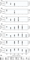
Algorithm response graphs separated by time to impact showing energy estimate variation based on distance to target for times to impact, $t_I$, of: a 1.563 s; b 1.875 s; c 2.344 s; d 3.125 s; e 4.688 s; f 6.251 s; g 9.376 s. h shows the distribution of relative background intensities. The different number of samples per time to impact is caused by not all distance and velocity pairs being present at all times to impact (refer to Sect. 3.4 for details). The lobula plate tangential cell (LPTC) model receptive field outputs have been normalised for display. Despite the varying distances to target, the distributions of the times to impact are statistically different. The statistical measure used (23) calculates based on the P5 (5th), P50 (50th, median), and P95 (95th) percentiles, which are indicated on the secondary y-axis and represented by horizontal dashed lines

Fig. 11

Region of interest responses for the output of each model within the proposed algorithm, against white (square markers), orange (diamond markers), and black (circle markers) backgrounds, for a distance of 200 mm and velocity of 127.98 mm/s ($t_I$ = 1.563 s): a The optical input to the algorithm; b The output of the photoreceptor (PR) model; c The output of the lamina monopolar cell (LMC) model; d The horizontal component of the output of the elementary motion detector (EMD) model; e The vertical component of the output of the EMD model, normalised the same as d to convey the lower signal magnitude of the vertical component; f The magnitude output of the medulla-lobula interneuron (MLI) model; and g The magnitude output of the lobula plate tangential cells (LPTC) model. All responses have been locally normalised for graphing purposes as their absolute signal magnitude is not of importance, just their statistical distribution. The LMC output (c) is not centred around 0 due to imperfect high-pass filtering. While the optical structure of the targets in (a) is similar, the responses of each model, especially the transition between background and target, are varied due to the drastic difference in background intensity, and hence contrast. Although the optical responses differ, the LPTC receptive field produces a very similar response for each background, although with some temporal misalignment present due to the adaptive filtering components of the algorithm. For best viewing, please see the online version of this article

Fig. 12

Component model responses at a distance of 200 mm, velocity of 127.98 mm/s ($t_I$ = 1.563 s), and for backgrounds: (C1) black; (C2) orange; and (C3) white. Model responses from processing frame index 0903 of the full recording have been rescaled, and the omnidirectional frame has been clipped to ±34${}^{\circ }$ horizontal field of view around the left perpendicular, for display purposes. All exposure values and post-processing gains for display were equal across all scenarios. Each row represents a different stage of the algorithm: (R1) optical input to the photoreceptor (PR) model; (R2) output of the PR model; (R3) output of the lamina monopolar cell (LMC) model; R4) horizontal component of the output of the elementary motion detector (EMD) model; (R5) vertical component of the output of the EMD model, shown at the same scale as R4 where, due to the purely horizontal motion, the columns will typically sum to an amplitude of 0; (R6) the magnitude output of the medulla-lobula interneuron (MLI) model, which features the novel contrast adaptation proposed in this research; and (R7) the output of the lobula plate tangential cell (LPTC) model prior to the receptive field window being sampled. The imperfect high-pass filtering in the LMC model is evident by a lack of sharp definition in the edges of R3. The aperture problem associated with the EMD is strongly illustrated in R4 and R5 where deep blue and white hot are opposite extremes of a custom colour scale. The benefit of moving to polar coordinates in the MLI is shown in R6 where only positive magnitudes (approaching white hot) are present. Despite the drastic difference in optical inputs (R1), and different structures within the EMD responses (R4 and R5), the adapted output of the MLI model (R6) and the corresponding spatio-temporal blur of the LPTC (R7) show similar responses across the 3 backgrounds. These results are spatial representations of the temporal results shown in Fig. 11, where $\sim i_{630}$ corresponds to the responses shown here

Fig. 13

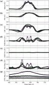
Region of interest responses for each model within the proposed algorithm for a black background at a velocity of 127.98 mm/s, for distances of 200 mm ($t_I$ = 1.563 s, dark purple, circle markers), 300 mm ($t_I$ = 2.344 s, dark green, diamond markers), 400 mm ($t_I$ = 3.125 s, light purple, square markers), and 600 mm ($t_I$ = 4.689 s, light green, plus markers): a Optical input; b Output of the photoreceptor (PR) model; c Output of the lamina monopolar cell (LMC) model; d Horizontal output of the elementary motion detector (EMD) model; e Vertical output of the EMD model, normalised per (d) to reflect the lower signal magnitude of the vertical component; f Output of the medulla-lobula interneuron (MLI) model; and g Output of the lobula plate tangential cell (LPTC) model. All responses were locally normalised as their absolute signal magnitude is not of importance, just their statistical distribution. The LMC output c is not centred around 0 due to imperfect high-pass filtering. Despite similarities between the peak amplitudes at the optical input, the LPTC is able to distinguish between the different times to impact caused by the different distances to the target. At the larger distances, the response to the target becomes less distinguishable compared to the background (see Fig. 7d). The different LPTC responses at the beginning (i500) and end (i775) are due to the different distances to the background; that is, the model is tracking the time to impact to the background, which is almost indistinguishable from the target at farther distances. For best viewing, please see the online version of this article

References

1. Arenz A, Drews M, Richter F, et al. The temporal tuning of the drosophila motion detectors is determined by the dynamics of their input elements. Curr Biol. 2017;27(7):929–944. doi: 10.1016/j.cub.2017.01.051. - DOI - PubMed
1. Babies B, Lindemann JP, Egelhaaf M, et al. Contrast-independent biologically inspired motion detection. Sensors. 2011;11(3):3303–3326. doi: 10.3390/s110303303. - DOI - PMC - PubMed
1. Bahl A, Serbe E, Meier M, et al. Neural mechanisms for Drosophila contrast vision. Neuron. 2015;88(6):1240–1252. doi: 10.1016/j.neuron.2015.11.004. - DOI - PubMed
1. Barron A, Srinivasan MV. Visual regulation of ground speed and headwind compensation in freely flying honey bees (ApisMellifera L.) J Exp Biol. 2006;209(5):978–984. doi: 10.1242/jeb.02085. - DOI - PubMed
1. Barth FG, Humphrey JA, Srinivasan MV. Frontiers in sensing: from biology to engineering. Amsterdam: Springer Science & Business Media; 2012.
Publication types
LinkOut - more resources