High-throughput automated methods for classical and operant conditioning of Drosophila larvae

Abstract

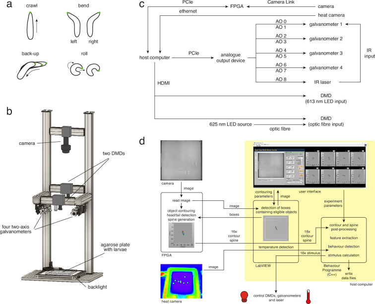
Learning which stimuli (classical conditioning) or which actions (operant conditioning) predict rewards or punishments can improve chances of survival. However, the circuit mechanisms that underlie distinct types of associative learning are still not fully understood. Automated, high-throughput paradigms for studying different types of associative learning, combined with manipulation of specific neurons in freely behaving animals, can help advance this field. The Drosophila melanogaster larva is a tractable model system for studying the circuit basis of behaviour, but many forms of associative learning have not yet been demonstrated in this animal. Here, we developed a high-throughput (i.e. multi-larva) training system that combines real-time behaviour detection of freely moving larvae with targeted opto- and thermogenetic stimulation of tracked animals. Both stimuli are controlled in either open- or closed-loop, and delivered with high temporal and spatial precision. Using this tracker, we show for the first time that Drosophila larvae can perform classical conditioning with no overlap between sensory stimuli (i.e. trace conditioning). We also demonstrate that larvae are capable of operant conditioning by inducing a bend direction preference through optogenetic activation of reward-encoding serotonergic neurons. Our results extend the known associative learning capacities of Drosophila larvae. Our automated training rig will facilitate the study of many different forms of associative learning and the identification of the neural circuits that underpin them.

Keywords: D. melanogaster; Drosophila melanogaster larva; behavior detection; closed-loop tracking; computational biology; computer vision; neuroscience; operant conditioning; stimulation; systems biology; trace conditioning.

Figure 1.. Multi-larva tracker combines real-time behaviour detection with either open- or closed-loop stimulation.

(a) Behavioural repertoire of Drosophila larvae. Schematics show the four most prominent actions displayed by Drosophila larvae (crawl, left and right bend, back-up, and roll). The larval contour is displayed as a black outline with a green dot marking the head. (b) Multi-larva tracker schematic showing the relative positions of the camera, digital micromirror devices (DMDs), galvanometers, agarose plate, and backlight. The heat camera is not shown (for visual simplicity), but is mounted directly beneath the background DMD. See multi-larva-tracker-cad.zip for technical drawings. (c) Block diagram of hardware components. AO: analogue output, FPGA: field-programmable gate array. d. Data flow between software elements.

Figure 1—figure supplement 1.. Contour calculation on eld-programmable gate array (FPGA).

A simplied example is shown using a 10 x 10 pixel box containing a small object. (a) The object (black) was detected against the background (white) using binary thresholding. Edge pixels were detected by combining the results of vertical and horizontal image convolution with a 2 x 1 XOR kernel using an OR operator. (b) The contour points were reconstructed in an iterative process, starting with the edge pixel closest to the centre of the box. The next contour point was defined as the first neighbouring pixel that was found to be an edge pixel. Neighbouring pixels were assessed clockwise from the pixel directly above the contour point. The process ended when no eligible edge pixels could be found.

Figure 1—figure supplement 2.. Detecting head and tail.

The larval contour (black outline) and head and tail (green) are shown. (a) Initial detection of head and tail. The head was the contour point with the sharpest curvature. The tail was the contour point with the next-sharpest curvature which did not lie in close proximity to the head. (b) The initial detection of head and tail was incorrect in some cases. False detection could be corrected by swapping head and tail, thereby minimising the distances from head and tail in the current frame (solid contour) to head and tail in the previous frame (transparent contour). (c) The correction described in b failed if larvae curled up such that the contour appeared circular (‘ball’). To eliminate this source of false head and tail detection, these events were detected using a ball classier.

Figure 1—figure supplement 3.. Calculating a smooth spine and landmark points.

The larval contour is shown (black outline). The spine S was comprised of 11 points (black), including head and tail (green). (a) The raw spine points were obtained by finding the centres between equally spaced contour points on either half of the contour as defined by head and tail. The first spine point was the head, the last spine point was the tail. (b) The smooth spine was obtained by exponentially smoothing the raw spine. (c) Four additional landmark points, neck_top, neck, and neck_down (blue), and the contour centroid (grey), were calculated.

Figure 1—figure supplement 4.. Calculating direction vectors.

Three direction vectors were calculated based on head, tail, and the landmark points. (a) direction_vector was the normalised vector from neck_down to neck. (b) direction_head_vector was the normalised vector from neck_top to head. (c) direction_tail_vector was the normalised vector from tail to neck_down.

Figure 1—figure supplement 5.. Features describing body shape.

(a) Outline of a larva with contour C (black) and its convex hull H (blue). (b) Shown here are the eigenvectors (blue) of the larval contour (black) structure tensor with respect to neck and their corresponding eigenvalues λ₁ and λ₂. (c) θ_i was defined as the angle between direction_vector (blue) and the vector ${\displaystyle {\overrightarrow{a}}_i}$ that passed through spine points Si and Si+1 (black). (d) θ_head was defined as the angle between direction_vector and direction_head_vector. Head and tail are shown in green.

Figure 1—figure supplement 6.. Velocity features.

The larval contour is shown in black while head and tail are shown in green. (a) crab_speed (blue) was defined as the component of neck_speed (grey) that was orthogonal to direction_vector_filtered (black). (b) parallel_speed (blue) was defined as the component of neck_speed_filtered (grey) that was parallel to direction_vector_ filtered (black). (c) parallel_speed_tail_raw (blue) was defined as the component of tail_speed_filtered (grey) that was parallel to direction_tail_vector_filtered (black). (d) θ_tail was defined as the angle between tail_speed_filtered (grey) and direction_tail_vector_filtered (black).

Figure 1—figure supplement 7.. Temporal smoothing of features.

(a-b) Example graphs of raw (dark blue) and filtered (mid blue) asymmetry (a) and eig_reduced (b) values over time. (c–d) Example graphs of raw (dark blue), filtered (mid blue), and long-time filtered (light blue) v_norm values over a short (c) and a long (d) period of time.

Figure 1—figure supplement 8.. Differentiation by convolution.

Example graphs of raw (dark blue) and convolved squared (green) asymmetry (a), eig_reduced (b), and v_norm (c) values over time.

Figure 2.. Optogenetic and thermogenetic stimulation efficiency verified by behavioural readout.

(a) Light stimulation hardware schematic. Only one digital micromirror device (DMD) is shown for simplicity. (b) Heat stimulation hardware schematic. Only one two-axis galvanometer is shown for simplicity. IR: infrared. (c) Proof-of-principle experiment protocol for either optogenetic (light bulb) or thermogenetic (thermometer) stimulation. d, e. Fraction of larvae for which the optogenetic (d) or thermogenetic (e) stimulus protocol triggered at least one detected roll (top pair of plots), bend (middle pair of plots), or forward crawl (bottom pair of plots). For each behaviour, the fraction of larvae is computed within 0.5 s (line plots) or 5 s (scatter plots) time bins across the 60 s experiment. All data shown with 95% Clopper-Pearson interval. Fisher’s exact test with Bonferroni correction was performed within each 5 s time bin between each experiment group (69F06 and 72F11) and the control group (attP2). Sample sizes for each genotype within each 5 s time bin are shown at the bottom of (d) and (e). ns p ≥ .05/24 (not significant), * p < .05/24, ** p < .01/24, *** p < .001/24. See Figure 2—source data 1, Figure 2—source data 2, Figure 2—source data 3.

Figure 2—figure supplement 1.. Temporal dynamics of larval heating via IR stimulation.

Larval temperature recorded before, during, and after delivery of 1470nm IR laser stimulation. Open-loop experiments began with a 30 s initialisation period during which no stimulus was given. Over a subsequent 20 s stimulation period (beginning at 0 s; grey vertical dashed line), a heat camera performed closed-loop adjustments of laser intensity to maintain the desired 30°C temperature (grey horizontal dashed line) at each larval location. The laser was then turned off to observe the time required for larvae to return to baseline temperature. Temperature readings were stopped 50 s after initial stimulus onset. Inset (grey solid rectangle) shows zoomed in temporal window for ease of visualisation. Temperature data were averaged across larvae (n = 36; data shown as mean ± 95% confidence interval). See Figure 2—source data 4.

Figure 3.. The effects of forward- versus backward-paired aversive training on larval attraction to Or42b.

(a) Schematic of classical conditioning protocol. After an initialisation period of 30 s, the first training round began. Here, Or42b was activated through red light illumination and was followed (forward-paired) or preceded (backward-paired) by the activation of Basin (72F11) neurons through heating. These stimuli were each delivered for 20 s, with a 5 s gap between them (i.e. inter-stimulus interval; ISI). A break of 60 s was allowed before the start of the next training round. In total, larvae completed eight training rounds (i.e. one training period). Larvae then completed a 60 s pre-test period without stimulation before the start of the testing period. The testing period comprised three testing rounds. During a single testing round, only Or42b was activated through red light illumination for 20 s, followed by a 45 s break. (b) Time-course of the percentage of experimental larvae bending during the testing period, averaged across all three testing rounds. Data were down-sampled from 20 Hz to 1 Hz to aid visualisation. Grey shading indicates the period of Or42b stimulation. Error shading shows the mean ± 95% confidence intervals (c) The average percentage of experimental larvae bending during the PRE (10–0 s before light onset), ON (0–20 s after light onset), and OFF (0–20 s after light offset) testing windows. Bars show medians, as well as upper and lower quartiles of data. (d, e) Data presented as in b and c, but for control larvae. (f) Percentage bending difference (ON-OFF) values after forward- and backward-paired training for both experimental and control larvae. Bars show medians, as well as upper and lower quartiles of data. Statistics calculated with a two-sided Mann-Whitney U test; * p < .01, *** p < .0001. See Figure 3—source data 1.

Figure 4.. Operant conditioning of bend direction in Drosophila larvae requires the ventral nerve cord.

(a) The goal of our automated operant conditioning paradigm is to reinforce an action of interest by coupling real-time behaviour detection with optogenetic activation of reward circuits. (b) High-throughput experiment protocol. During training, each larva (black contour with green head) received optogenetic stimulus (red light bulb) when bent to one predefined side (depicted as left), and no stimulus otherwise (grey light bulb). (c–h) Gal4 expression is depicted as color-coded CNS (see legend). UAS-CsChrimson effector abbreviated as CsChr for visual clarity. Bars show medians, as well as upper and lower quartiles of data. Outliers (filled diamonds) are randomly jittered horizontally to aid visualisation. (c–f) top row. Larval bend rate shown as number of bends per minute, grouped by bends to stimulated side (dark red) or unstimulated side (grey). For larvae that received random, uncorrelated stimulation during 50% of bends (d), left and right bend rate are shown in light red. Statistical comparisons calculated using a paired, two-sided Wilcoxon signed-rank test. (c–f) bottom row. Difference in bend rate (black) shown between the stimulated and unstimulated sides or, in the case of the uncorrelated training group (panel d), between left and right sides. Statistical comparisons calculated using a two-sided Wilcoxon signed-rank test. (c–f). Data shown from the test periods before training round 1 (Before) and after training round 4 (After). n is the number of larvae in each time bin. Exact p-values written above corresponding data. ns p ≥ .05 (not significant), * p < .05, ** p < .01, *** p < .001. (g). Bend rate data after training round 4 (same data as in (c) and (d) top row), with bend rate for uncorrelated training group calculated without stratification by bend direction. Statistics calculated with a two-sided Mann-Whitney U test, with Bonferroni correction; ns p ≥ .05/2 (not significant), ** p < .01/2. (e) Difference in bend rate after training round 4 (same data as in c–f bottom row). Statistical comparisons against Ddc > CsChr calculated with a two-sided Mann-Whitney U test, with Bonferroni correction; * p < .05/3, ** p < .01/3. See Figure 4—source data 1.

Figure 4—figure supplement 1.. Ddc-Gal4 expression pattern without and with tsh-Gal80 restriction.

Maximum intensity projections of confocal images obtained after immunohistochemical staining. Plan-Apochromat 20x objective, resolution: 592 x 800 pixels, scale bar: 100 μm. Images courtesy of the HHMI Janelia FlyLight team. (a, e) (green in d and h). Targeting a green fluorescent protein (GFP) antibody to the mVenus tag of CsChrimson. (b, f) (red in d and h). Staining against BP104. (c, g) (blue in d and h) Staining against N-cadherin. (a–d) Ddc>CsChrimson larvae. Manually counting the cell bodies in the image stacks revealed more than 200 GFP-positive neurons located in the brain, subesophageal zone (SEZ), and ventral nerve cord (VNC), including the PAM cluster dopaminergic neurons innervating the mushroom body (n = 2). This confirmed that Ddc- Gal4 drives broad expression across the central nervous system (CNS) ( Li et al., 2000; Lundell and Hirsh, 1994). (e–h) Ddc>CsChrimson, tsh>Gal80 larvae. As expected, no GFP-positive neurons were found in the VNC (n = 6). Ddc brain and SEZ expression remained largely unaffected by Gal80, as the GFP-positive neurons in both areas that could be consistently identified in Ddc>CsChrimson larvae (n = 3) were also present in Ddc>CsChrimson, tsh>Gal80 larvae (n = 3).

Figure 4—figure supplement 2.. Drosophila larvae show bend direction preference during operant paradigm training.

High-throughput experiments followed the protocol depicted in Figure 4B. Gal4 expression depicted as color-coded CNS (see legend). UAS-CsChrimson effector abbreviated as CsChr for visual clarity. Data shown in 1 min time bins (separated by vertical dashed lines) across the entire experiment, beginning with the test period before training round 1 and ending with the test period after training round 4. Larval bend rate shown as number of bends per minute, grouped by bends to stimulated side (dark red) or unstimulated side (dark grey). For larvae that received random, uncorrelated stimulation during 50% of bends (panel b), left and right bend rate are shown in light red. Bars show medians, as well as upper and lower quartiles of data. Outliers (open diamonds) are randomly jittered horizontally to aid visualisation. Number of larvae in each time bin is written just below the x-axis. Exact p-values written above corresponding data. Statistical comparisons calculated using a paired, two-sided Wilcoxon signed-rank test. ns p ≥ .05 (not significant), * p < .05, ** p < .01, *** p < .001. See Figure 4—source data 1.

Figure 4—figure supplement 3.. Operant conditioning of bend direction in Drosophila larvae with single-larva tracker.

(a) Software framework of single-larva tracker. Still images from the graphical user interface show aerial views of a single Drosophila larva in the behaviour arena (blue outline: contour; head: green dot; tail: red dot; green words: detected behaviours). (b) Hardware schematic for optogenetic stimulation. System hardware was nearly identical to that described in Schulze et al., 2015. A camera and an IR backlight, both mounted on motorised linear slides, tracked the real-time behaviours of a single larva moving along a stationary agarose plate. When a chosen behaviour was detected, the red LED turned on, stimulating the larva. (c) Experiment protocol using the single-larva closed-loop tracker. Behaviours are depicted as larval contours (black) with head (green dot). During training, the larva received optogenetic stimulus (red light bulb) when bent to one predefined side (depicted as left), and no stimulus otherwise (grey light bulb). (d, e, f) Gal4 expression depicted as color-coded CNS (see legend). UAS-CsChrimson effector abbreviated as CsChr for visual clarity. Bars show medians, as well as upper and lower quartiles of data. Outliers (filled diamonds) are randomly jittered horizontally to aid visualisation. d, e top row. Larval bend rate shown as number of bends per minute, grouped by bends to stimulated side (dark red) or unstimulated side (grey). Statistical comparisons calculated using a paired, twosided Wilcoxon signed-rank test. (d, e) bottom row. Difference in bend rate (black) between the stimulated and unstimulated sides. Statistical comparisons calculated using a two-sided Wilcoxon signed-rank test. (d–e) Data shown from the test periods before training round 1 (Before) and after training round 2 (After). n is the number of larvae in each time bin. Exact p-values written above corresponding data. ns p ≥ 0.05 (not significant), * p < 0.05, ** p < 0.01. f. Difference in bend rate after training round 2 (same data as in d and e bottom row). Statistical comparison between genotypes calculated using a two-sided Mann-Whitney U test. * p < 0.05. See Figure 4—source data 2.

Figure 5.. Serotonergic neurons may mediate operant conditioning.

High-throughput experiments followed the protocol depicted in Figure 4B. Gal4 expression is depicted as color-coded CNS (see legend). UAS-CsChrimson effector abbreviated as CsChr for visual clarity. Bars show medians, as well as upper and lower quartiles of data. Outliers (filled diamonds) are randomly jittered horizontally to aid visualisation. (a–c) top row. Larval bend rate shown as number of bends per minute, grouped by bends to stimulated side (dark red) or unstimulated side (grey). Statistical comparisons calculated using a paired, two-sided Wilcoxon signed-rank test. (a–c) bottom row. Difference in bend rate (black) shown between the stimulated and unstimulated sides. Statistical comparisons calculated using a two-sided Wilcoxon signed-rank test. (a–c). Data shown from the test periods before training round 1 (Before) and after training round 4 (After). n is the number of larvae in each time bin. Exact p-values written above corresponding data. ns p ≥ .05 (not significant), * p < .05. (d) Difference in bend rate after training round 4 (same data as in a–c bottom row). Statistical comparisons against Tph > CsChr calculated with a two-sided Mann-Whitney U test, with Bonferroni correction; ns p ≥ .05/2 (not significant), * p < .05/2. See Figure 5—source data 1.

Figure 5—figure supplement 1.. Tph-Gal4 expression pattern without and with tsh-Gal80 restriction.

Maximum intensity projections of confocal images obtained after immunohistochemical staining. Plan-Apochromat 20x objective, resolution: 592 x 800 pixels, scale bar: 100 μm. Images courtesy of the HHMI Janelia FlyLight team. (a–d) Tph>CsChrimson larvae, (e–h) Tph>CsChrimson, tsh>Gal80 larvae. (a, e) (green in d and h). Staining against green fluorescent protein (GFP) antibody targeting the mVenus tag of CsChrimson. (b, f) (red in d and h). Staining against BP104. (c, g) (blue in d and h). Staining against N-cadherin.

References

1. Abramson CI, Dinges CW, Wells H, Nieh JC. Operant conditioning in honey bees (Apis mellifera L.): the cap pushing response. PLOS ONE. 2016;11:e0162347. doi: 10.1371/journal.pone.0162347. - DOI - PMC - PubMed
1. Aceves-Piña EO, Quinn WG. Learning in normal and mutant Drosophila larvae. Science. 1979;206:93–96. doi: 10.1126/science.206.4414.93. - DOI - PubMed
1. Alexander J, Audesirk TE, Audesirk GJ. One-trial reward learning in the snail lymnea stagnalis. Journal of Neurobiology. 1984;15:67–72. doi: 10.1002/neu.480150107. - DOI - PubMed
1. Andreatta M, Pauli P. Appetitive vs. aversive conditioning in humans. Frontiers in Behavioral Neuroscience. 2015;9:128. doi: 10.3389/fnbeh.2015.00128. - DOI - PMC - PubMed
1. Apostolopoulou AA, Mazija L, Wüst A, Thum AS. The neuronal and molecular basis of quinine-dependent bitter taste signaling in Drosophila larvae. Frontiers in Behavioral Neuroscience. 2014;8:6. doi: 10.3389/fnbeh.2014.00006. - DOI - PMC - PubMed
Publication types
MeSH terms
LinkOut - more resources