Reaction-diffusion models in weighted and directed connectomes

Abstract

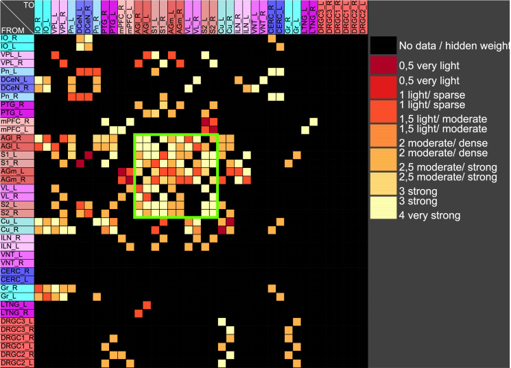
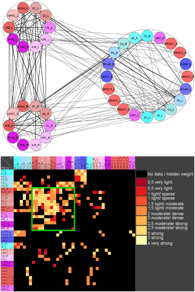
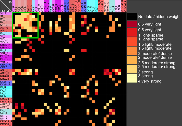
Connectomes represent comprehensive descriptions of neural connections in a nervous system to better understand and model central brain function and peripheral processing of afferent and efferent neural signals. Connectomes can be considered as a distinctive and necessary structural component alongside glial, vascular, neurochemical, and metabolic networks of the nervous systems of higher organisms that are required for the control of body functions and interaction with the environment. They are carriers of functional phenomena such as planning behavior and cognition, which are based on the processing of highly dynamic neural signaling patterns. In this study, we examine more detailed connectomes with edge weighting and orientation properties, in which reciprocal neuronal connections are also considered. Diffusion processes are a further necessary condition for generating dynamic bioelectric patterns in connectomes. Based on our precise connectome data, we investigate different diffusion-reaction models to study the propagation of dynamic concentration patterns in control and lesioned connectomes. Therefore, differential equations for modeling diffusion were combined with well-known reaction terms to allow the use of connection weights, connectivity orientation and spatial distances. Three reaction-diffusion systems Gray-Scott, Gierer-Meinhardt and Mimura-Murray were investigated. For this purpose, implicit solvers were implemented in a numerically stable reaction-diffusion system within the framework of neuroVIISAS. The implemented reaction-diffusion systems were applied to a subconnectome which shapes the mechanosensitive pathway that is strongly affected in the multiple sclerosis demyelination disease. It was found that demyelination modeling by connectivity weight modulation changes the oscillations of the target region, i.e. the primary somatosensory cortex, of the mechanosensitive pathway. In conclusion, a new application of reaction-diffusion systems to weighted and directed connectomes has been realized. Because the implementation was realized in the neuroVIISAS framework many possibilities for the study of dynamic reaction-diffusion processes in empirical connectomes as well as specific randomized network models are available now.

Fig 1. The weighted adjacency matrix of a bilateral mechanosensory subconnectome.

The weighted adjacency matrix of the spinal cord, brainstem, diencephalic and cortical connectivity of the mechanosensory pathways. The last character of the area abbreviation indicates the side of the hemisphere: L: left hemisphere, R: right hemisphere. AGl: Lateral agranular prefrontal cortex, AGm: Medial agranular prefrontal cortex, CERC: Cerebellar cortex, Cu: Cuneate nucleus, DCeN: Cerebellar nuclei, DRGC1: Dorsal root ganglion of cervical segment 1, DRGC2: Dorsal root ganglion of cervical segment 2, DRGC3: Dorsal root ganglion of cervical segment 3, Gr: Gracile nucleus principal part, ILN: Intralaminar nuclei, IO: Inferior olive, LTNG: Lateral thalamic nuclear group, mPFC: Medial prefrontal cortex, Pn: Pontine nuclei, PTG: Posterior group, S1: Primary somatosensory cortex, S2: Secondary somatosensory cortex, VL: Ventrolateral thalamic nucleus, VNT: Ventral thalamus, VPL: Ventral posterolateral thalamic nucleus.

Fig 2. The weighted digraph of the bilateral mechanosensory subconnectome.

The bilateral weighted digraph of the adjacency matrix shown in Fig 1. The dashed lines indicate contralateral projections.

Fig 3. Functions of concentrations for regions of left side.

The functions of concentrations of left hemispheric regions are shown for the GM RD-model. Initial conditions V₀ = 1 and W₀ = 1 were set for the dorsal root ganglia of the left side. The color coding of the functions in this diagram and all following function representations in diagram form are based on the color definition in the area hierarchy, which is simplified in the adjacency matrix in Fig 1. Thus, the colors of the columns and rows of the adjacency matrix represent the color scale of the functions. The x-axis shows the iteration steps of the function. On the y-axis the diffused concentrations are shown according to the applied models and functions. These axis assignments were also maintained uniformly for all subsequent function diagrams.

Fig 4. Relation of average concentrations and local network parameters.

a) The correlation c = 0.726 of average concentrations (AvgGEMEx) and the CluC_Out ($\frac{D{G}_{in}}{D{G}_{a}ll}$) coefficient. b) Each point indicates the rank of a local network parameter of a region. The green curve represents the mean ranks. The colors correspond to the color assignments to the considered regions of the network, which were introduced in Fig 1 in the form of an adjacency matrix.

Fig 5. Average cross-correlation matrix of four parameters of the GM model.

The average cross-correlation matrix of the variation of the four reaction constants is shown. This matrix has been used for further cluster analysis.

Fig 6. Average cross-correlation matrix of two reaction constants.

The average cross-correlation of the variation of the two reaction constants has been analyzed by spectral clustering. A coherent group of regions (green rectangle) could be determined.

Fig 7. Average cross-correlation matrix of four parameters.

The average cross-correlation of the variation of the two reaction constants and the two decay parameters for activators and inhibitors has been analyzed by spectral clustering. A similar group of regions (green rectangle) could be determined as found with a two parameter variation.

Fig 8. Average cross-correlation matrix of four parameters of the MM model.

The average cross-correlation of the variation of four reaction parameters is shown. Large positive correlation values close to 1 indicate a strong similarity of concentrations of a pair of regions.

Fig 9. Spectral cluster analysis of the average cross-correlation matrix of the variation of four parameters of the MM model.

The average cross-correlation of the variation of the four reaction parameters has been analyzed by spectral clustering. A similar group of regions (green rectangle) could be determined as found with the GM parameter variation.

Fig 10. Modularity and spectral cluster analysis.

The modularity analysis of connectivity similarity among regions generates 3 modules. The spectral cluster analysis of the connectivity matching matrix reveal a cluster with similar regions like those of the clustered cross-correlation matrices.

Fig 11. Similarities of clusterings referring GM parameter variation.

The reaction parameters and decay rates for substances A and B were varied 256 times. a) RD functions of all regions using default parameters. b) Similarities of the clusterings using spectral clustering (Light: high similarity, dark low similarity). c) Similarities of the clusterings using Markov clustering (Light: high similarity, dark low similarity). d) Magnification of upper left corner of the matrix in b). e) Magnification of upper left corner of the matrix in c).

Fig 12. Similarities of clusterings referring MM parameter variation.

The reaction parameters A-D were varied 375 times. a) RD functions of all regions using default parameters. b) Similarities of the clusterings using spectral clustering (Light: high similarity, dark low similarity). c) Similarities of the clusterings using Markov clustering (Light: high similarity, dark low similarity). d) Magnification of upper left corner of the matrix in b). e) Magnification of upper left corner of the matrix in c).

Fig 13. Result of clustering the cross-correlation matrix of a GM process.

The somatosensory regions constitute a cluster (green rectangle).

Fig 14. Result of clustering the cross-correlation matrix of a MM process.

The somatosensory regions are contained in the same cluster like in the GM model.

Fig 15. Linear stability analysis of the GM model.

The curve shows where the real part of the first eigenvalue of the Jacobian matrix in the fix-point is zero in dependence of the parameters a (sigmaa) and b (mua).

Fig 16. Stability of function u and v.

a) The GM model was applied to exactly one non-connected node to show that the function u has a stable progression above a certain number of iterations. The function of u for a = b = 0.01 shows stability at about 100 iterations. b) For the same parameters as given before, the function v is given.

Fig 17. Real part of first eigenvalue of the GM model.

The real parts of the first eigenvalue of the Jacobian matrix in dependence of the parameters a (sigmaa) and b (mua).

Fig 18. Oscillations of functions u and v.

a) In addition to the stability of the function u in Fig 16 the regularity of the oscillations shall be shown here. The regularity extends over all performed iterations. b) The regularity of the oscillations of the function v is shown here. As with the function u, the regularity extends over all iterations performed.

Fig 19. Weight modulation function.

This weight modulation function (damped cosine function) is applied to the GM RD-system. Initial conditions V₀ = 1 and W₀ = 1 were set for the dorsal root ganglia of the left side.

Fig 20. Weight modulation function.

The weight modulation function (damped cosine function) is applied to the GM RD-system. Initial conditions V₀ = 1 and W₀ = 1 were set for the dorsal root ganglia of the left side. The number of iterations is 10000. The amplitudes were fixed to 10 and the lower value of the weight reduction was set to 0.1.

Fig 21. The weight modulation function.

This weight modulation function (damped cosine function) is applied to the MM RD-system. It has the same scale of time like the MM RD simulation.

Fig 22. Adjacency matrix.

Adjacency matrix of mechanosensitive subnetwork.

Fig 23. Network representation of the adjacency matrix.

The network of the adjacency matrix of Fig 22 is visualized.

References

1. Deco G, Jirsa VK, McIntosh AR. Resting brains never rest: computational insights into potential cognitive architectures. Trends Neurosci. 2013; 36: 268–274. doi: 10.1016/j.tins.2013.03.001 - DOI - PubMed
1. Turing AM. The chemical basis of morphogenesis. Phil Trans R Soc Lond B. 1952; 237: 37–72. doi: 10.1098/rstb.1952.0012 - DOI
1. Prigogine I, Lefever R. Symmetry breaking instabilities in dissipative systems. J Chem Phys. 1968; 48: 1695–1700. doi: 10.1063/1.1668896 - DOI
1. Castets V, Dulos E, Boissonade J, De Kepper P. Experimental evidence of a sustained standing Turing-type nonequilibrium chemical pattern. Phys Rev Lett. 1990; 64: 2953–2956. doi: 10.1103/PhysRevLett.64.2953 - DOI - PubMed
1. Ouyang Q, Swinney HL. Transition from an uniform state to hexagonal and striped Turing patterns. Nature 1991; 352: 610–612. doi: 10.1038/352610a0 - DOI
Publication types