A Mathematical Description of the Flow in a Spherical Lymph Node

Abstract

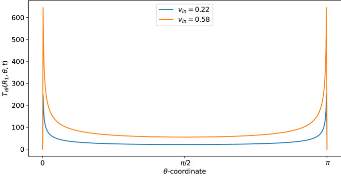
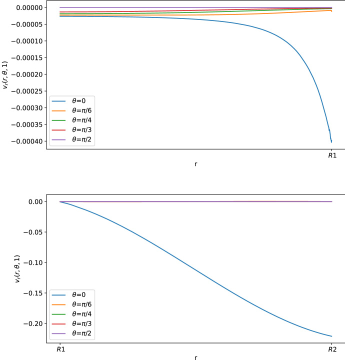
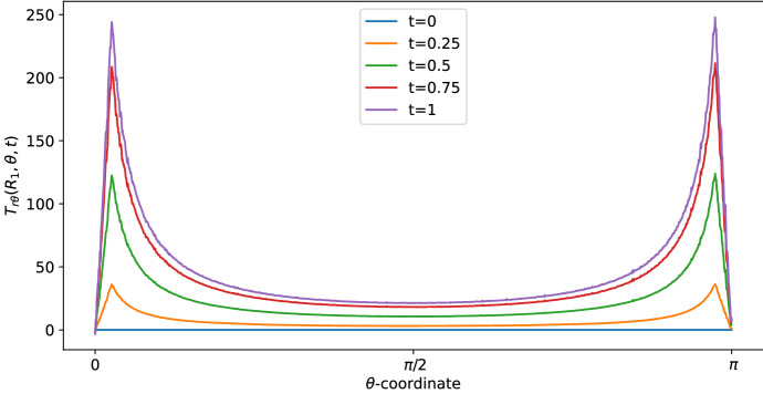
The motion of the lymph has a very important role in the immune system, and it is influenced by the porosity of the lymph nodes: more than 90% takes the peripheral path without entering the lymphoid compartment. In this paper, we construct a mathematical model of a lymph node assumed to have a spherical geometry, where the subcapsular sinus is a thin spherical shell near the external wall of the lymph node and the core is a porous material describing the lymphoid compartment. For the mathematical formulation, we assume incompressibility and we use Stokes together with Darcy-Brinkman equation for the flow of the lymph. Thanks to the hypothesis of axisymmetric flow with respect to the azimuthal angle and the use of the stream function approach, we find an explicit solution for the fully developed pulsatile flow in terms of Gegenbauer polynomials. A selected set of plots is provided to show the trend of motion in the case of physiological parameters. Then, a finite element simulation is performed and it is compared with the explicit solution.

Keywords: Darcy–Brinkman equation; Lymph node; Pulsatile flow; Spherical domain.

Fig. 1

Pressure distribution in mPa with fixed pressure $p=6.18\times {10}^5$ mPa at the outlet (color figure online)

Fig. 2

Shear stress $T_{r\theta }(r,\theta ,t)$ in mPa with respect to the polar angle ($\theta =0$ near the inlet flow and $\theta =\pi$ near the outlet flow) calculated at $t=1$ s and in the internal radius $R_1$ with different boundary velocities in mm/s (where $v_{\text{in}}\approx 0.22$ corresponds to $L={10}^{-3}{\text{mm}}^3$/s and $v_{\text{in}}\approx 0.58$ corresponds to $L=2.2\times {10}^{-3}{\text{mm}}^3$/s) (color figure online)

Fig. 3

Tangential component of the velocity in mm/s with respect to the radius at different angles at $t=1$ s. The first picture corresponds to the tangential velocity in the LC (porous part), and the second corresponds to the tangential velocity in the SCS (free-fluid region) (color figure online)

Fig. 4

Normal component of the velocity in mm/s with respect to the radius at different angles at $t=1$ s (color figure online)

Fig. 5

Tangential component of the velocity in mm/s with respect to the radius at different angles at $t=1$ s. The first graph corresponds to the tangential velocity in the LC (porous part), and the second corresponds to the tangential velocity in the SCS (free-fluid region) (color figure online)

Fig. 6

Normal component of the velocity in mm/s with respect to the radius at different angles at $t=1$ s. The first graph corresponds to the tangential velocity in the LC (porous part), and the second corresponds to the tangential velocity in the SCS (free-fluid region) (color figure online)

Fig. 7

Shear stress in mPa with respect to the polar coordinates calculated at a fixed radius $r=R_1$ in different times (color figure online)

Fig. 8

Pressure distribution in mPa with fixed pressure $\overline{p}=6.18\times {10}^5$ mPa at outlet (color figure online)

Fig. 9

Shear stress in mPa with respect to the polar angle ($\theta =0$ near the inlet flow and $\theta =\pi$ near the outlet flow) calculated at different times (color figure online)

Fig. 10

Velocity magnitude in mm/s at $t=1$ s (maximum velocity) (color figure online)

Fig. 11

Tangential component of the velocity in mm/s with respect to the radius at different angles at $t=1$ s. The first graph corresponds to the tangential velocity in the LC (porous part), and the second corresponds to the tangential velocity in the SCS (free-fluid region) (color figure online)

References

-
- Abramowitz M, Stegun IA. Handbook of mathematical functions with formulas, graphs, and mathematical tables. Washington: US Government Printing Office; 1964.
- Adair TH, Guyton AC. Modification of lymph by lymph nodes. II. Effect of increased lymph node venous blood pressure. Am J Physiol Heart Circul Physiol. 1983;245(4):616–622. - PubMed
- Adair TH, Guyton AC. Modification of lymph by lymph nodes. III. Effect of increased lymph hydrostatic pressure. Am J Physiol Heart Circul Physiol. 1985;249(4):777–782. - PubMed
- Angot P. Well-posed Stokes/Brinkman and Stokes/Darcy coupling revisited with new jump interface conditions. ESAIM: Math Model Numer Anal. 2018;52(5):1875–1911.
- Angot P, Goyeau B, Ochoa-Tapia JA. Asymptotic modeling of transport phenomena at the interface between a fluid and a porous layer: jump conditions. Phys Rev E. 2017;95(6):063302. - PubMed
Publication types
MeSH terms
LinkOut - more resources
Full Text Sources