A round-robin approach provides a detailed assessment of biomolecular small-angle scattering data reproducibility and yields consensus curves for benchmarking

Abstract

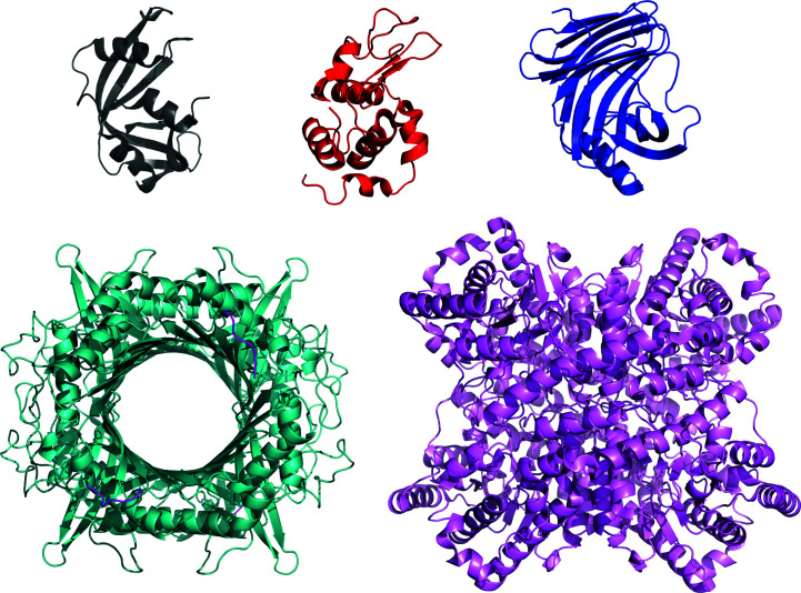
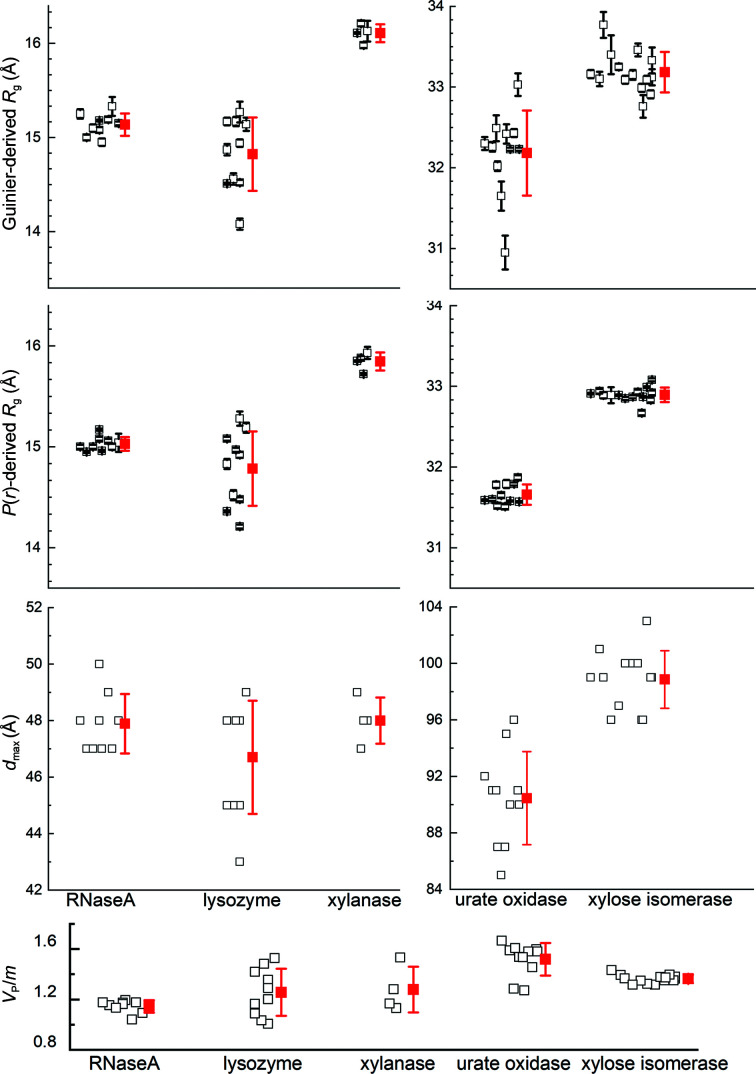
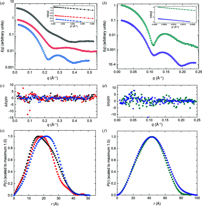
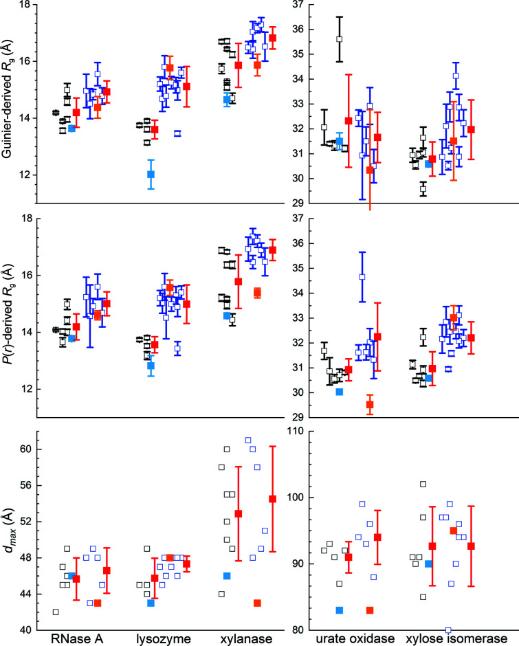
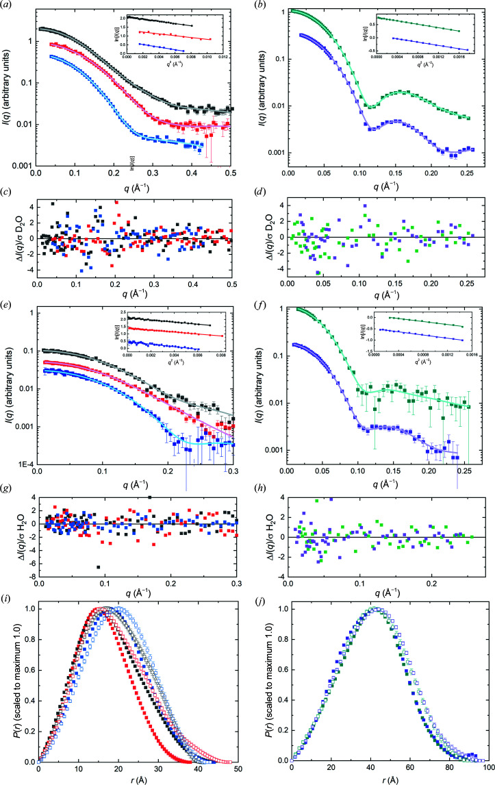
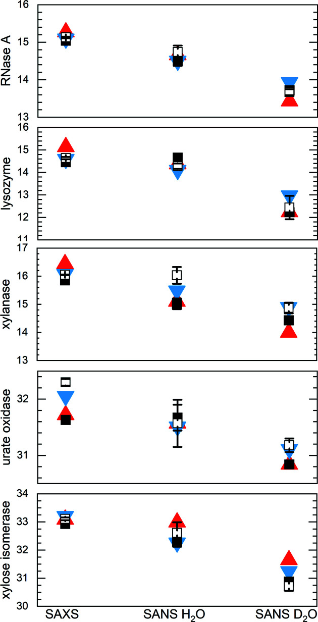
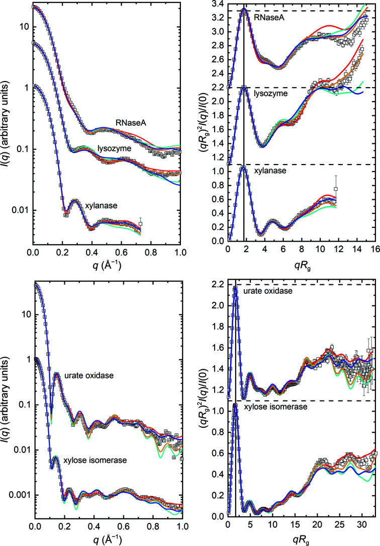
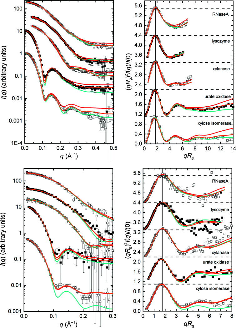
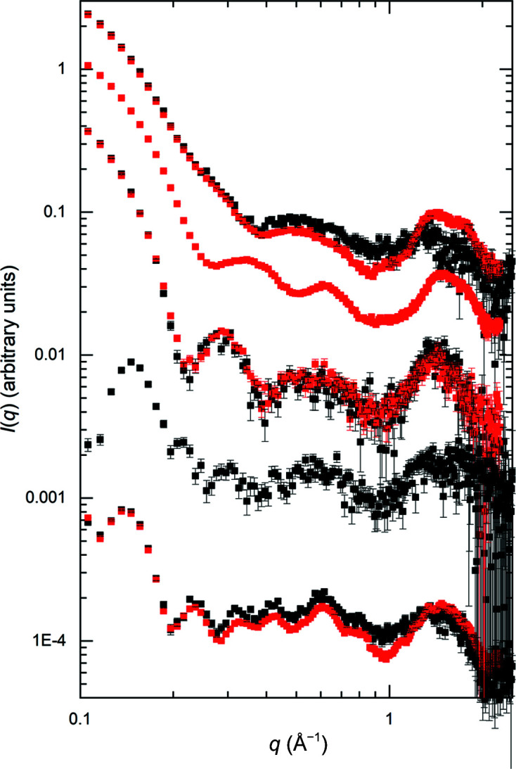
Through an expansive international effort that involved data collection on 12 small-angle X-ray scattering (SAXS) and four small-angle neutron scattering (SANS) instruments, 171 SAXS and 76 SANS measurements for five proteins (ribonuclease A, lysozyme, xylanase, urate oxidase and xylose isomerase) were acquired. From these data, the solvent-subtracted protein scattering profiles were shown to be reproducible, with the caveat that an additive constant adjustment was required to account for small errors in solvent subtraction. Further, the major features of the obtained consensus SAXS data over the q measurement range 0-1 Å^-1 are consistent with theoretical prediction. The inherently lower statistical precision for SANS limited the reliably measured q-range to <0.5 Å^-1, but within the limits of experimental uncertainties the major features of the consensus SANS data were also consistent with prediction for all five proteins measured in H₂O and in D₂O. Thus, a foundation set of consensus SAS profiles has been obtained for benchmarking scattering-profile prediction from atomic coordinates. Additionally, two sets of SAXS data measured at different facilities to q > 2.2 Å^-1 showed good mutual agreement, affirming that this region has interpretable features for structural modelling. SAS measurements with inline size-exclusion chromatography (SEC) proved to be generally superior for eliminating sample heterogeneity, but with unavoidable sample dilution during column elution, while batch SAS data collected at higher concentrations and for longer times provided superior statistical precision. Careful merging of data measured using inline SEC and batch modes, or low- and high-concentration data from batch measurements, was successful in eliminating small amounts of aggregate or interparticle interference from the scattering while providing improved statistical precision overall for the benchmarking data set.

Keywords: X-ray scattering; benchmarking standards; biomolecular small-angle scattering; neutron scattering; scattering-profile calculation; standards.

Figure 1

Ribbon representations of the crystal structures of RNaseA (PDB entry 7rsa, black), lysozyme (PDB entry 2vb1, red), xylanase (PDB entry 2dfc, blue), urate oxidase (PDB entry 3l8w, dark cyan, with added C-terminal SLKSKL in magenta) and xylose isomerase (PDB entry 1mnz, purple).

Figure 2

Distribution of Guinier and P(r)-derived R _g values, d _max values and the Porod volume to molecular mass ratio (V _P/m) for the data contributing to the consensus SAXS profiles for each protein. Individual experimental values are represented as black open squares, with horizontal offsets for clarity and error bars for R _g values (standard errors). Red squares represent the mean values for each set, with error bars indicating ±1 standard deviation.

Figure 3

(a, b) I(q) versus q for consensus SAXS data (symbols) for each protein with P(r) model fits (lines). Insets are Guinier plots to qR _g = 1.3. (c, d) Error-weighted residual plots for the P(r) model fits in (a) and (b), respectively. (e, f) P(r) versus r corresponding to the fits in (a) and (b), respectively. Error bars are standard errors, and where not apparent are smaller than the symbols. The colour key for the symbols throughout is RNaseA, black; lysozyme, red; xylanase, blue; urate oxidase, dark cyan; xylose isomerase, purple.

Figure 4

Distribution of Guinier- and P(r)-derived R _g values and associated d _max values for SANS measurements for each protein in D₂O (batch data, open black squares; SEC–SANS data, light blue filled squares) and H₂O (batch data, open blue squares; SEC–SANS data, orange filled squares) with horizontal offsets for clarity. Errors bars on individual R _g values are standard errors. Red squares represent the mean value for each set, with the error bar indicating ±1 standard deviation. The values for H₂O urate oxidase SEC–SANS are for data that have a constant additive background adjustment to match the batch data.

Figure 5

(a, b) I(q) versus q (symbols) with P(r) model fits (black lines) from consensus SANS data in D₂O for each protein, with Guinier plots (to qR _g = 1.3) as insets. (c, d) Error-weighted residual plots for the fits in (a) and (b), respectively. (e) and (f) are the same plots as in (a) and (b) but for SANS data in H₂O, with (g) and (h) showing the corresponding error-weighted residual plots. (i, j) Corresponding P(r) versus r plots for the fits in (a) and (b) (D₂O, solid squares) and (e) and (f) (H₂O, open squares). The colour key throughout is RNaseA, black; lysozyme, red; xylanase, blue; urate oxidase, dark cyan; xylose isomerase, purple. Error bars are standard errors, and where not apparent are smaller than the symbols.

Figure 6

Guinier- and P(r)-derived R _g values (open and filled black squares, respectively) for RNaseA, lysozyme, xylanase, urate oxidase and xylose isomerase consensus profiles for SAXS, SANS in H₂O and SANS in D₂O measurements (Tables 2 ▸ and 3 ▸) compared with R _g values predicted with CRYSOL/CRYSON (red filled triangles) and WAXSiS (blue filled inverted triangles) (Supplementary Table S8). Where they are not evident, error bars for R _g from the consensus curve are smaller than the symbols.

Figure 7

I(q) versus q and dimensionless Kratky [(qR _g)² I(q)/I(0) versus qR _g] plots for the consensus data (open black squares) overlaid with the profiles predicted by WAXSiS (red), CRYSOL (cyan), Pepsi-SAXS (orange) and FoXS (blue) from the crystal structures. Every second or third experiment point is omitted for clarity. I(q) versus q plots are offset vertically, while the Kratky plots are stacked vertically so that for each panel the dashed lines are for (qR _g)² I(q)/I(0) = 0.0 or 1.1 for the plots above or below, respectively. The solid black reference lines in the Kratky plots are at qR _g = 1.73. Error bars are standard errors based on propagated counting statistics.

Figure 8

I(q) versus q and dimensionless Kratky [(qR _g)² I(q)/I(0) versus qR _g] plots for the consensus SANS data (black squares) in D₂O (upper plots) or H₂O (lower plots) overlaid with the profiles predicted by WAXSiS (red), CRYSON (cyan) and Pepsi-SANS (orange) from the crystal structures. I(q) versus q plots are offset vertically for clarity; from top to bottom, RNaseA, lysozyme, xylanase, urate oxidase and xylose isomerase. Kratky plots are stacked vertically so that for each panel the dashed lines are for (qR _g)² I(q)/I(0) = 0.0 or 1.1 for the plots above or below, respectively. Black solid reference lines in the Kratky plots are at qR _g = 1.73. Error bars are standard errors based on propagated counting statistics.

Figure 9

Data for (top to bottom traces) RNaseA, lysozyme, xylanase, urate oxidase and xylose isomerase from SEC–WAXS (black symbols, measured on the P12 BioSAXS beamline at EMBL, no lysozyme data) and batch WAXS (red symbols, measured on the 12-ID-B beamline at the APS, no urate oxidase data). The plot is log–log, with every second data point skipped for the sake of clarity and starting at q = 0.1 Å⁻¹ to better highlight the data beyond q = 1 Å⁻¹. Full log–log and log linear plots are given in Supplementary Fig. S12. Error bars are standard errors based on propagated counting statistics.

References

1. Abraham, M. J., Murtola, T., Schulz, R., Páll, S., Smith, J. C., Hess, B. & Lindahl, E. (2015). SoftwareX, 1–2, 19–25.
1. Basham, M., Filik, J., Wharmby, M. T., Chang, P. C. Y., El Kassaby, B., Gerring, M., Aishima, J., Levik, K., Pulford, B. C. A., Sikharulidze, I., Sneddon, D., Webber, M., Dhesi, S. S., Maccherozzi, F., Svensson, O., Brockhauser, S., Náray, G. & Ashton, A. W. (2015). J. Synchrotron Rad. 22, 853–858. - PMC - PubMed
1. Berendsen, H. J. C., Postma, J. P. M., van Gunsteren, W. F., DiNola, A. & Haak, J. R. (1984). J. Chem. Phys. 81, 3684–3690.
1. Bernadó, P., Mylonas, E., Petoukhov, M. V., Blackledge, M. & Svergun, D. I. (2007). J. Am. Chem. Soc. 129, 5656–5664. - PubMed
1. Blanchet, C. E., Spilotros, A., Schwemmer, F., Graewert, M. A., Kikhney, A., Jeffries, C. M., Franke, D., Mark, D., Zengerle, R., Cipriani, F., Fiedler, S., Roessle, M. & Svergun, D. I. (2015). J. Appl. Cryst. 48, 431–443. - PMC - PubMed