MOSAICS: A software suite for analysis of membrane structure and dynamics in simulated trajectories

Abstract

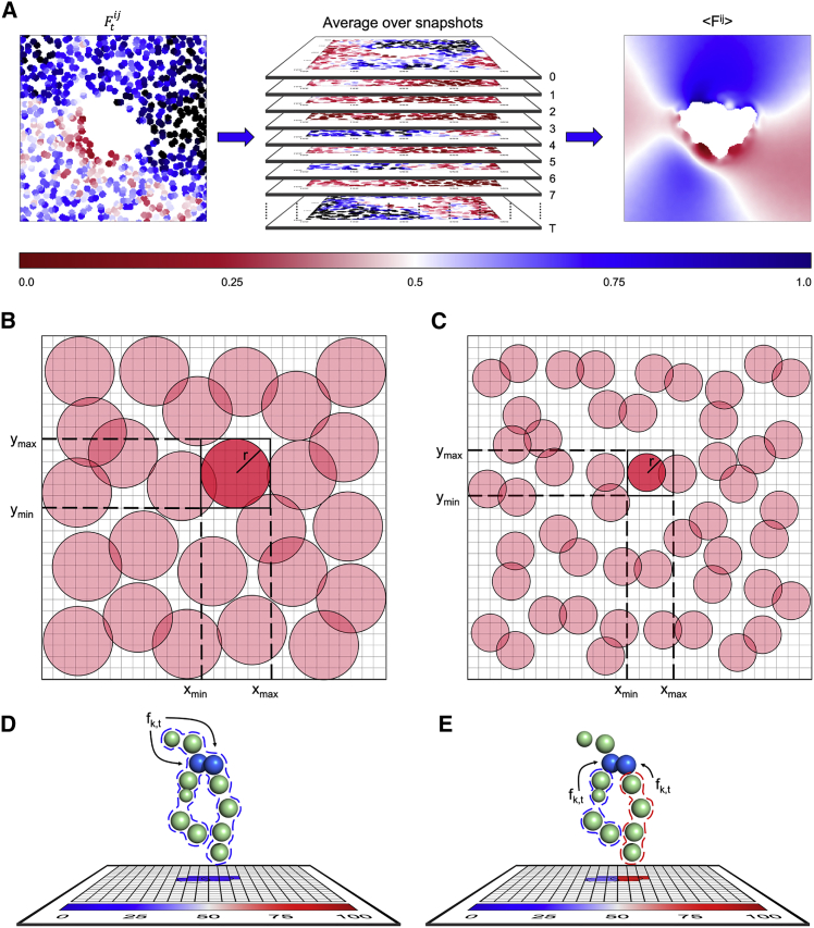
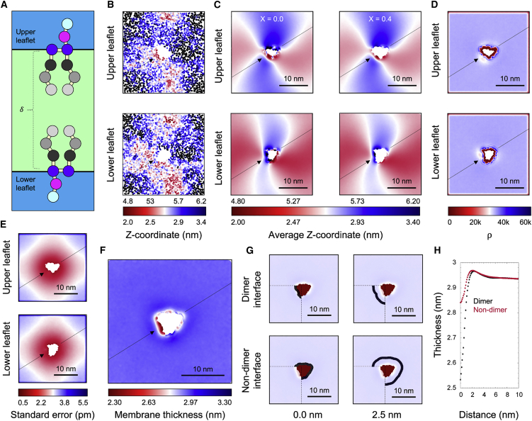
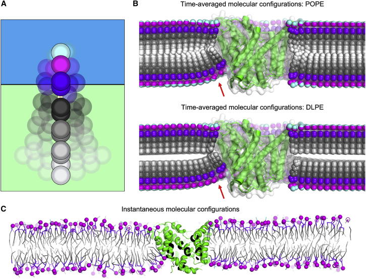
Molecular dynamics (MD) simulations have become the predominant computational analysis method in membrane biophysics, as this technique is uniquely suited for investigations of complex molecular systems through the relevant physical principles. Owing to continued improvements in scope and performance, the trajectories generated through this approach contain ever-increasing amounts of information, which must be synthesized and simplified in post-analysis using tools that are not only mechanistically insightful but also computationally efficient and highly scalable. Here, we introduce MOSAICS, a self-contained high-performance suite of C++ software tools designed for advanced analyses of lipid bilayer structure and dynamics from MD trajectories. MOSAICS is to our knowledge the most comprehensive software suite of this kind, enabling analysis of a wide array of morphological and kinetic properties, for both simple and complex membranes, irrespective of system size or resolution. Importantly, MOSAICS is designed to provide spatial distributions of all computed quantities, with built-in masking tools, noise filtering, and statistical significance metrics to facilitate quantitative interpretations of the trajectory data; it is also fully parallelized and can therefore leverage the capabilities of supercomputing facilities. Despite its technical sophistication, MOSAICS is user-friendly and requires minimal computational expertise, making it accessible to researchers of all skill levels. This sofware suite can be freely downloaded at https://github.com/MOSAICS-NIH/.

Figure 1

MOSAICS workflows and procedures. (A) For each individual trajectory snapshot, the stamping interpolation method is used to map a specific characteristic or observable onto a two-dimensional lattice (left). The data are then averaged over all snapshots (middle) to give $\langle F^{ij}\rangle$ (right). In this example the white area in the center of the lattice is occupied by the protein, and the color bar specifies the value of the observable. (B) Schematic of the stamping method for a simple case where each lipid position in XY is represented by a single mapping atom. In this example, the mapping atoms are represented as red circles whose radius matches the would-be stamping radius. A single lipid is selected (dark red) and the bounds for which lipid-to-grid-point distances must be measured are indicated via the enclosed box and dotted lines. (C) Same schematic as in (B) when multiple mapping atoms are selected instead to improve the spatial resolution of the data. As in (B), the mapping atoms are represented with red circles; we focus on a single mapping atom to highlight the neighboring lattice points for which distances must be measured. (D and E) Schematic of the procedure used for mapping observables onto the lattice. In these examples, the mapping atoms are colored in blue. (D) Shows an example where a single observable is measured for the whole molecule as is indicated by the dotted lines. In this case, the measurement is assigned to each of the two mapping atoms. In contrast, (E) exemplifies a case where two different chemical groups (each of the acyl chains) are characterized, again indicated by dotted lines; in this case, each of these measurements are assigned to a single mapping atom.

Figure 2

MOSAICS workflows and procedures. (A) Criteria used by the “leaflet finder” to assign lipids to the upper or lower leaflets of the bilayer. An assignment number is computed for each lipid molecule by subtracting the values of the Z-coordinate of two atoms, one in the headgroup and another in the acyl chain, as indicated in the diagram. A positive value identifies lipids in the upper leaflet while a negative number identifies those in the lower leaflet. (B) Top, schematic of a rectangular selection tool. In this example, we have selected a square membrane patch surrounding the protein (central region colored white) from a map containing membrane thickness data. The resulting rectangle is drawn in red with the enclosed area shaded. Bottom, an example of a lattice point selection made with a masking tool. Here, we have selected the protein from the upper panel. (C) Schematic of a noise filter. For descriptors that rely on hard thresholds, it is common that rapid fluctuations result in spurious assignments; in this example, the value of a certain observable $O_k$ in snapshot t is an outlier among the values observed for the snapshots that precede and follow t, leading the noise filter to reassign this value. (D) Common command line arguments used when launching a MOSAICS tool. Note that the atom selections are made using a selection card, i.e., a formatted text file. (E) Flow chart depiction of the lattice-based procedure employed by MOSAICS. Input files are colored in cyan. The main loop, which runs over a subset of the trajectory snapshots assigned to an MPI process, is highlighted in blue.

Figure 3

Membrane shape and thickness. (A) Schematic of a thickness measurement using the Z-coordinate of pseudoatoms GL1 and GL2 from each leaflet, which represent the ester linkages in a coarse-grained phospholipid structure. (B) Stamping interpolation map of the Z-coordinate used for thickness measurements taken from the first trajectory snapshot. (C) Time average of the Z-coordinate of the same atoms examined in (B), before and after excluding lattice points whose sample count is below 40% of the global average. (D) Map of the sample count that describes the number of snapshots for which each lattice point was characterized after stamping. (E) Standard error of the mean for the Z-coordinate map shown in (C). (F) Membrane thickness estimated as the distance separating the upper and lower surfaces in (C). (G) Masks used for selecting grid points to be averaged when computing the membrane thickness as a function of distance to the protein surface. Each mask, i.e., a selection shell with a width of 1 nm, is shown in black with the distance between the shell midplane and the protein (shown in red) indicated below the plot. For clarity, the thickness data that are averaged are shown as a transparent overlay. (H) Average membrane thickness computed as a function of the distance to the protein surface, using the masks depicted in (G). Note that the data shown in (B–H) describe all lipid types in the system, i.e., POPE, POPG, DLPE, and DLPG; spatial distributions in this and subsequent figures were obtained using a 28 × 28 nm lattice with a lattice point spacing of 0.7 Å, and a stamping radius of 0.23 nm. Note in (B and C) upper and lower leaflets are plotted on different scales, specified by the numeric values above and below the corresponding color bars. In this and subsequent figures the CLC dimerization interface is indicated with an arrow and the axis perpendicular to this interface is marked with a line passing through the protein.

Figure 4

Internal lipid structure and leaflet entanglement. (A) Time-averaged map of the acyl chain end-to-end length, shown as δ in the corresponding schematic, as measured by the distance separating the pseudoatoms GL1/GL2 and C4A/C4B. (B) Time-averaged map of the second-rank order parameter, averaged over all pseudobonds in each acyl-chain. (C) Time-averaged map of the lipid tilt angle relative to the z axis (Eq. 13). (D) Time-averaged map of the number of interleaflet contacts per lipid. In this example, contacts are counted between the two groups of atoms enclosed by the dotted lines as indicated by red arrows. Note that the data shown in (A–D) describe POPE and POPG lipids only, for clarity.

Figure 5

Average lipid configurations. (A) Schematic of the time averaging of instantaneous lipid configurations. Note that the rotational freedom and internal dynamics of lipid molecules cause the average configuration to resemble a (non-physical) linear structure perpendicular to the membrane midplane, with both acyl chains superposed and in line with the headgroup. (B) Average configurations for POPE and DLPE lipids. Despite the fact that the single-molecule averages are non-physical structures, this representation clearly illustrates the nature of the membrane deformations induced by the protein, and the impact of DL lipids on membrane thickness. Regions containing highly tilted lipids whose lipid heads groups fan outwards are indicated with a red arrow. The average protein structure is also shown alongside, with secondary structure elements in green and the surface in white. (C) One of the snapshots of the trajectory analyzed in (B), shown in cross section for clarity. The dimensions of the simulation system are 28 × 28 nm, including ∼2600 lipid molecules.

Figure 6

Descriptors of lipid density and lipid-type enrichment. (A) Time-averaged map of the number of lipid-nearest neighbors, measured for the headgroup layer. The geometric center for each headgroup is indicated by a green circle. (B) Left, Voronoi diagrams computed for a single trajectory snapshot; right, time-averaged map of area per lipid. (C) Time-averaged map of the alkyl chain hydration number. Water molecules are represented as red circles in the corresponding schematic and the contacts with the lipid by dotted lines. (D) Enrichment factor computed for DL lipids. Note that the data shown in (A–C) describe all lipid types in the system, i.e., POPE, POPG, DLPE, and DLPG.

Figure 7

Lipid mixing and self-diffusion. (A) Schematic of a lipid solvation shell of radius $R_{ss}$ around the lipid geometric center (green circles), in this case computed using the GL1 and GL2 pseudoatoms. (B) The number of lipids found in the first solvation shells of a set of target lipids is given as a function of time. (C) Probability distribution of the single-molecule residence time in those solvation shells; the average residence time is indicated. (D) Percentage of lipids in the bilayer that (transiently) visit the first solvation shells of the target lipids, i.e., the mixing fraction. In (B and C) error bars represent the variance across lipid molecules (Eq. 19). The noise filter used in this analysis encompasses 3 ns of simulation time, and the first solvation shell was defined as having a radius of 1.1 nm. (E) Schematic of lipid diffusion; the position of each lipid is tracked by the X- and Y-coordinates of a geometric center, indicated by a green circle. (F) Mean-square displacement (MSD) of either POPE/POPG lipids (left) or DLPE/DLPG lipids (right), as a function of the elapsed time τ. Black lines represent the MSD for all lipids of each type, while the gray lines represent the MSD of individual lipids; the red dotted line represents a linear regression of all the data, which was used to derive the diffusion coefficient, $D$, using Eq. 21.

Figure 8

Residence time analyses. (A) Noise filtering of Voronoi diagrams used to calculate two-dimensional maps of the lipid dwell time in different regions of the membrane. (B) Two-dimensional distributions of the mean residence time for PO and DL lipids. (C) Assignment of lipids to solvation shells around the protein, defined separately for the CLC dimerization interface and the rest of the protein surface. The first-shell lipids are colored cyan, while second, third, fourth, and fifth shells are colored purple, green, yellow, and red, respectively; subsequent solvation shells are colored white. (D) Probability distributions of the residence time in the first lipid solvation shell, either for PO or DL lipids, either at the dimerization interface or elsewhere. Average residence times are indicated in each case. The noise filter used in this analysis encompasses 3 ns of simulation time.

Figure 9

Computing performance and scalability. (A) Spatially resolved distributions for four different descriptors of membrane structure, calculated with MOSAICS or LiPyphilic. The descriptors are: bilayer shape, quantified by the mean Z-coordinate of the GL1/GL2 pseudoatoms; the area per lipid in the plane of the phosphate atoms; the second-rank order parameter, averaged over each acyl chain; and the mean instantaneous tilt angle of the chains, measured for a the GL1-C4A and GL2-C4B atom pairs (calculated with the “P2” tool in the case of MOSAICS). (B) Clock times required to obtain the results shown in (A), normalized by the number of snapshots in the trajectory. For MOSAICS, timings are given for calculations carried out on a single CPU core as well as over 10, 100, and 500 CPU cores of the same type. For LiPyphilic, which to our knowledge does not currently support parallelization, timings for single-core calculations are provided. (C) Evaluation of the membrane shape for a system containing a cluster of 37 copies of the ATG9A trimeric protein. (D) Clock times required to obtain the results shown in (C), presented as in (B).

References

1. Allen W.J., Lemkul J.A., Bevan D.R. GridMAT-MD: a grid-based membrane analysis tool for use with molecular dynamics. J. Comput. Chem. 2009;30:1952–1958. - PubMed
1. Carr M., MacPhee C.E. Membrainy: a ‘smart’ unified membrane analysis tool. Source Code Biol. Med. 2015;10:3. - PMC - PubMed
1. Lukat G., Krüger J., Sommer B. APL@Voro: a Voronoi-based membrane analysis tool for GROMACS trajectories. J. Chem. Inf. Model. 2013;53:2908–2925. - PubMed
1. Ramasubramani V., Dice B.D., et al. Glotzer S.C. Freud: a software suite for high throughput analysis of particle simulation data. Comput. Phys. Commun. 2020;254:107275.
1. Romo T.D., Leioatts N., Grossfield A. Lightweight object-oriented structure analysis: tools for building tools to analyze molecular dynamics simulations. J. Comput. Chem. 2014;35:2305–2318. - PMC - PubMed
Publication types
LinkOut - more resources