. 2022 Nov 5;84(12):144.
doi: 10.1007/s11538-022-01102-7.

Effect of Human Behavior on the Evolution of Viral Strains During an Epidemic

Affiliations

Effect of Human Behavior on the Evolution of Viral Strains During an Epidemic

Asma Azizi et al. Bull Math Biol. .

Abstract

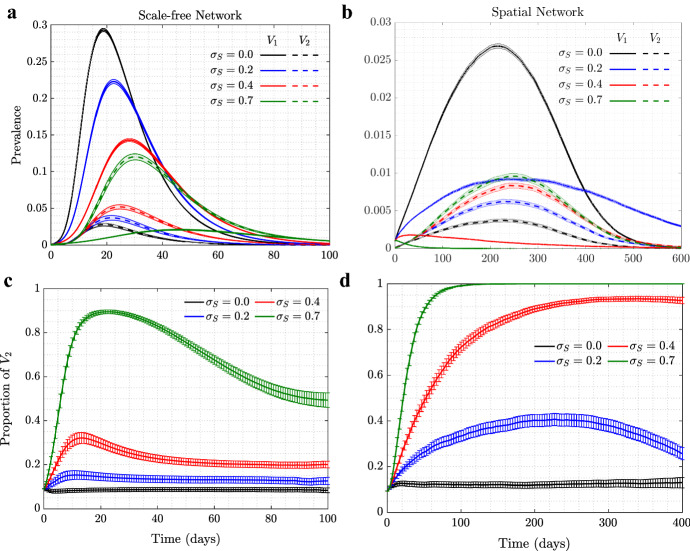
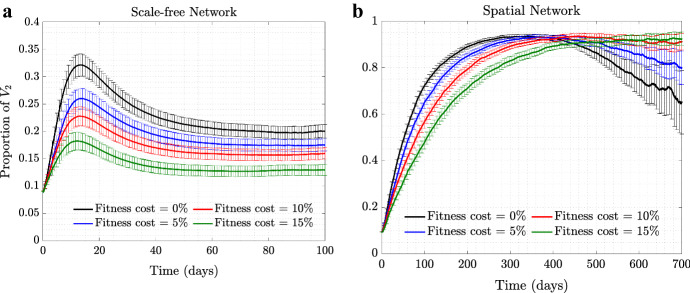
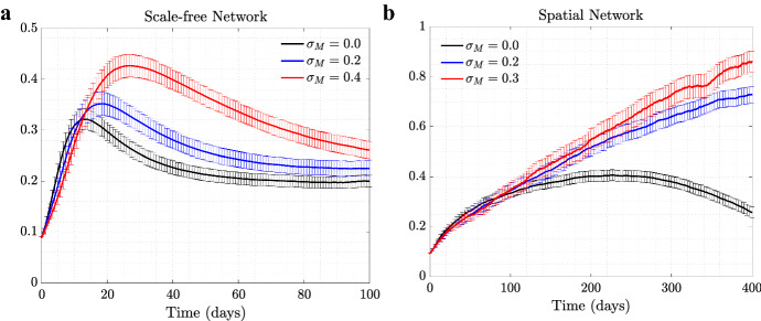
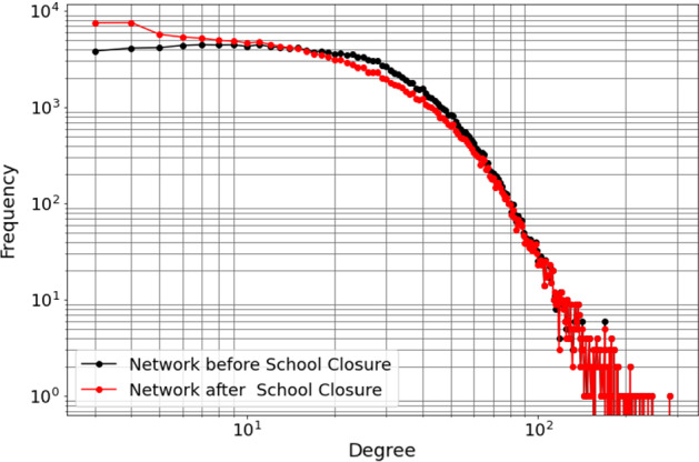
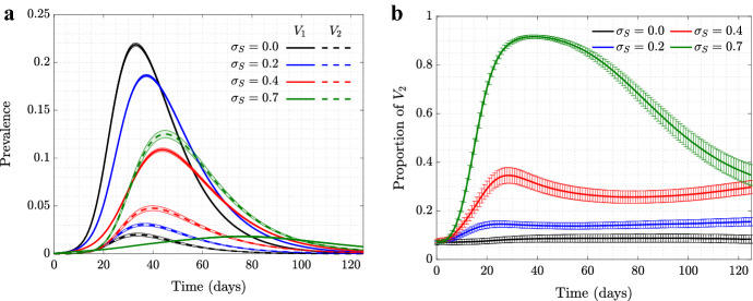
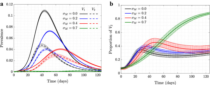
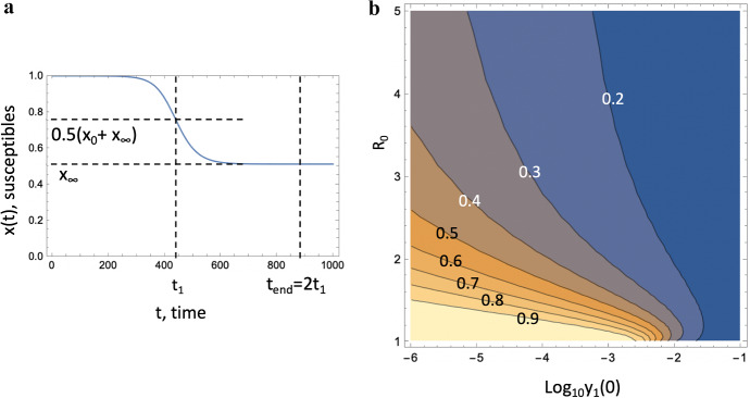
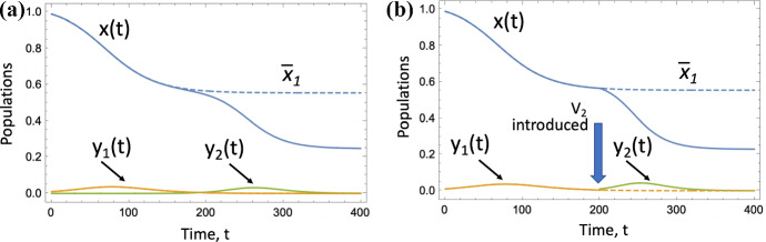
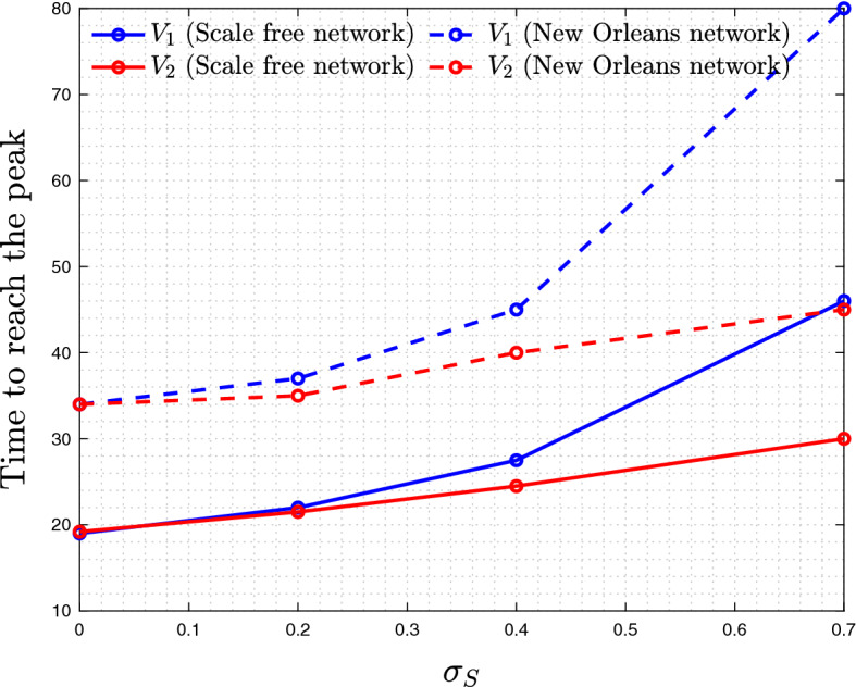
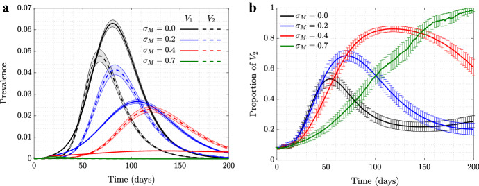
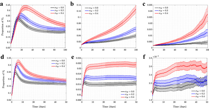
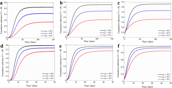
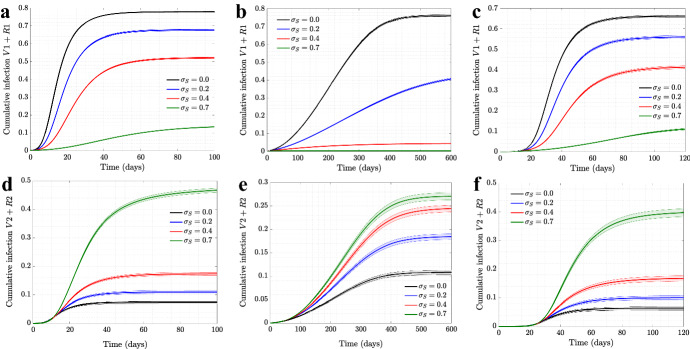
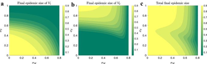
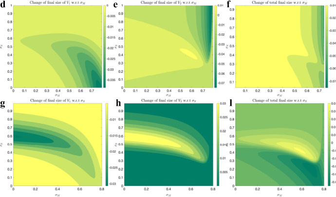
It is well known in the literature that human behavior can change as a reaction to disease observed in others, and that such behavioral changes can be an important factor in the spread of an epidemic. It has been noted that human behavioral traits in disease avoidance are under selection in the presence of infectious diseases. Here, we explore a complementary trend: the pathogen itself might experience a force of selection to become less "visible," or less "symptomatic," in the presence of such human behavioral trends. Using a stochastic SIR agent-based model, we investigated the co-evolution of two viral strains with cross-immunity, where the resident strain is symptomatic while the mutant strain is asymptomatic. We assumed that individuals exercised self-regulated social distancing (SD) behavior if one of their neighbors was infected with a symptomatic strain. We observed that the proportion of asymptomatic carriers increased over time with a stronger effect corresponding to higher levels of self-regulated SD. Adding mandated SD made the effect more significant, while the existence of a time-delay between the onset of infection and the change of behavior reduced the advantage of the asymptomatic strain. These results were consistent under random geometric networks, scale-free networks, and a synthetic network that represented the social behavior of the residents of New Orleans.

Keywords: Asymptomatic variant; Mandated social distancing; Network; Self-regulated social distancing; Symptomatic variant; Viral evolution.


Figures

Fig. 1
Fig. 1
(Color figure online) The role of self-regulated SD in the spread of viruses. Time series are shown for four scenarios: No (σS=0, black), low (σS=0.2, blue), moderate (σS=0.4, red), and high (σS=0.7, green) self-regulated SD, and in the absence of mandated SD. Scale-free (left) and spatial (right) networks of 10, 000 individuals with average degree 10 are used. a, b The prevalence of V1 (solid) and V2 (dashed); c, d the proportion of V2 (V2/(V1+V2)). The remaining parameters are γ+δ=0.1 per day, ψ=0.0012, β1=β2=0.028 per day per contact for the scale-free and β1=β2=0.037 per day per contact for the spatial network (corresponding to R0=2.5). Means and standard errors are shown for 5000 stochastic realizations
Fig. 2
Fig. 2
(Color figure online) Selection for V2 in the presence of a fitness cost. Time series of proportion of V2 under moderate self-regulated SD, σS=0.4 (and with σM=0), are shown for 0% fitness cost (β2=β1, black), 5% fitness cost (β2=0.95β1, blue), 10% fitness cost (β2=0.9β1, red), and 15% fitness cost (β2=0.85β1, green), for a scale-free and b spatial networks. All the other parameters are as in Fig. 1
Fig. 3
Fig. 3
(Color figure online) The effect of mandated SD on the proportion of V2. The proportion of the asymptomatic strain, V2, is shown as a function time, for three different levels of mandated SD: a Scale-free network, σM=0 (black), σM=0.2 (blue), and σM=0.4, with σS=0.4; b spatial network, σM=0 (black), σM=0.2 (blue), and σM=0.3 (red), with σS=0.2. All the other parameters are as in Fig. 1. The levels for mandated and self-regulated SD are selected in such a way that R0 remains above one so an outbreak for V1 is observed
Fig. 4
Fig. 4
(Color figure online) The effect of delay of self-regulated SD on selection of V2. The proportion of V2 is shown as time series for the a scale-free and b spatial network, in the presence of time delay in the appearance of symptoms when infected by V1. The different colors correspond to time delays of 0, 1, , 5 days. Here, σS=0.4, σM=0.0, and the rest of the parameters are as in Fig.  1
Fig. 5
Fig. 5
(Color figure online) Degree distribution of the New Orleans synthetic network. Red: the basic network; black: the network under school closure (see “Appendix 3”). The network includes 150, 000 nodes and has average degree 15.82 (with average degree 12.67 under school closure)
Fig. 6
Fig. 6
(Color figure online) New Orleans Network of size 150, 000 individuals: the role of self-regulated SD in the spread of viruses. Time series are shown for four scenarios of no (σS=0, black), low (σS=0.2, blue), moderate (σS=0.4, red), and high (σS=0.7, green) self-regulated SD, in the absence of mandated SD. a plot is the prevalence of V1 (solid) and V2 (dashed); b shows the proportion of V2 (V2/(V1+V2)). β1=β2=0.2 and all the other parameters are as in Fig. 1 (corresponding to R0=2.5). Means and standard errors are shown for 1000 stochastic realizations
Fig. 7
Fig. 7
(Color figure online) New Orleans Network of size 150, 000 individuals: the role of mandated SD in the spread of viruses. Time series are shown for four scenarios of no (σM=0, black), low (σM=0.2, blue), moderate (σM=0.4, red), and high (σM=0.6, green) mandated SD, in the presence of moderate self-regulated SD (σS=0.4). a plot is the prevalence of V1 (solid) and V2 (dashed); b shows the proportion of V2 (V2/(V1+V2)). β1=β2=0.2 and all the other parameters are as in Fig. 1 (corresponding to R0=2.5). Means and standard errors are shown for 1000 stochastic realizations
Fig. 8
Fig. 8
Fraction of an advantageous virus, V2. a The quantity z(t) obtained by solving Eqs. (1–1c) is plotted as a function of time for several values of R0, obtained by changing the death rate, a. b The corresponding susceptible populations as functions of time. The rest of the parameters are β1=0.1,β2=0.11,y1(0)=0.001,y2(0)=0.1y1(0)
Fig. 9
Fig. 9
(Color figure online) Fraction of V2 at the end of the epidemic. a Calculation of tend, which represents the end of the epidemic, is illustrated. The blue line is the fraction of susceptible individuals, x(t), obtained as a solution of Eqs. (1–1c); tend=2t1, where t1 corresponds to x(t1)=12(x(0)+x). In other words, at time t1 the population of susceptible individuals reaches halfway to its final value, x. b Quantity y2/(y1+y2) obtained by solving Eqs. (1–1c), is plotted at time tend, as a function of the initial proportion of individuals infected with V1, and R0. The rest of the parameters are β1=0.1,β2=0.11,y2(0)=0.1y1(0)
Fig. 10
Fig. 10
Illustration of time-separated epidemics. a Numerical solution of system (1–1c) with initial conditions y10=0.01,y20=10-8,x0=1-y10-y20, where the mutant infection is characterized by an initial condition much lower than that of the wild type. The three populations are plotted as a function of time. The dashed lines show the system behavior in the absence of the mutant, and in particular, the quantity x¯1 is shown. b Numerical solutions of system (–) with y1(0)=0.01 for t[0,T] and system (8–10) with y2(T)=0.01 for t>T. The other parameters are β1=0.13,β2=2β1,γ=0.1,T=200
Fig. 11
Fig. 11
(Color figure online) Time to reach infection peak for viruses V1 (blue) and V2 (red), as a function of σS (the measure of V2 advantage)
Fig. 12
Fig. 12
(Color figure online) New Orleans Network under school closure: the role of self-regulated SD in the spread of viruses. Time series are shown for four scenarios of no (σS=0, black), low (σS=0.2, blue), moderate (σS=0.4, red), and high (σS=0.7, green) self-regulated SD, in the absence of mandated SD. a Plot is the prevalence of V1 (solid) and V2 (dashed); b shows the proportion of V2 (V2/(V1+V2)). β1=β2=0.29 and all the other parameters are as in Fig.  1 in the main text (corresponding to R0=2.5). Means and standard errors are shown for 1000 stochastic realizations
Fig. 13
Fig. 13
(Color figure online) New Orleans Network under school closure: the role of mandated SD in the spread of viruses. Time series are shown for four scenarios of no (σM=0, black), low (σM=0.2, blue), moderate (σM=0.4, red), and high (σM=0.6, green) mandated SD, in the presence of moderate self-regulated SD (σS=0.4). a plot is the prevalence of V1 (solid) and V2 (dashed); b shows the proportion of V2 (V2/(V1+V2)). β1=β2=0.29 and all the other parameters are as in Fig.  1 in the main text (corresponding to R0=2.5). Means and standard errors are shown for 1000 stochastic realizations
Fig. 14
Fig. 14
The effect of mandated SD on the proportion of V2 for scenarios of low/high transmission rate and different initial conditions. The proportion of the asymptomatic strain, V2, is shown as a function time, for 3 different levels of mandated SD (σM=0,0.2,0.4) and fixed positive level of self-regulated SD (σS=0.4) on scale-free network: a β=0.0028 per day and V2(0)V1(0)=0.1; b β=0.0028 per day and V2(0)V1(0)=0.01; c β=0.0028 per day and V2(0)V1(0)=0.002; d β=0.1 per day and V2(0)V1(0)=0.1; e β=0.1 per day and V2(0)V1(0)=0.01; and f β=0.1 per day and V2(0)V1(0)=0.002. All the other parameters are as in Fig. 1. The levels for mandated and self-regulated SD are selected in such a way that R0 remains above one so an outbreak for V1 is observed
Fig. 15
Fig. 15
The effect of mandated SD on cumulative infection of symptomatic strain for scenarios of low/high transmission rate and different initial conditions. The cumulative infection for symptomatic strain, V1+R1, is shown as a function time, for six different levels of mandated SD (σM=0,0.2,0.4) and fixed positive level of self-regulated SD (σS=0.4) on scale-free network. The parameters for af are as in Fig.  14
Fig. 16
Fig. 16
The effect of mandated SD on cumulative infection of asymptomatic strain for scenarios of low/high transmission rate and different initial conditions. The cumulative infection for asymptomatic strain, V2+R2, is shown as a function time, for six different levels of mandated SD (σM=0,0.2,0.4) and fixed positive level of self-regulated SD (σS=0.4) on scale-free network. The parameters for af are as in Fig.  14
Fig. 17
Fig. 17
The effect of self-regulated SD on cumulative infection of symptomatic/asymptomatic strains for various network structures. The cumulative infections for are shown as a function time, for four different levels of self-regulated SD (σS=0,0.2,0.4,0.7) and no mandated SD (σM=0.0), simulated on a, d scale-free network; b, e spatial network; c, f New Orleans network. All the other parameters are as in Fig.  1 for ae and Fig. 6 for c, f
Fig. 18
Fig. 18
Final sizes versus SD levels: the model in (1–1c) is used to quantify the amount of final sizes for V1 (a), V2 (b), and both (c), for different levels of SD strategies (σM and σS). The parameter values are β=0.5, γ=0.1, and for initial condition we have y10=0.05 and y20=0.0001, thus y20y10=0.002
Fig. 19
Fig. 19
Change in final sizes with respect to SD levels: The same model and parameter values as the one in Fig.  (18) are used to quantify the change of final sizes with respect change of SD strategies
Fig. 20
Fig. 20
The region for which final epidemic sizes increase as a result of social distancing, for various transmission rates: The same model and recovery rate as those in Fig.  (18), initial condition y10=0.001, y20=0.0001 (y20y10=0.1), and various transmission rates are used. The left column shows the region of SD parameter values, for which final epidemic size of V2 increases with increasing mandated SD. The right column shows the region of SD parameter values, for which total final epidemic size increases with increasing self-regulated SD
Fig. 21
Fig. 21
The region for which final epidemic sizes increase as a result of social distancing for various initial conditions: The same model and infection parameters as those in Fig.  (18), but various initial conditions are used. The left column shows the region of SD parameter values, for which final epidemic size of V2 increases with increase in mandated SD. The right column shows the region of SD parameter values, for which total final epidemic size increases with increase in self-regulated SD

Similar articles

Cited by

References

    1. Anderson RM, May RM. Infectious diseases of humans: dynamics and control. Oxford: Oxford University Press; 1992.
    1. Andersson-Ellström A, Forssman L, Milsom I. The relationship between knowledge about sexually transmitted diseases and actual sexual behaviour in a group of teenage girls. Sex Transm Infect. 1996;72(1):32–36. - PMC - PubMed
    1. Ariful Kabir KM, Kuga K, Tanimoto J. Effect of information spreading to suppress the disease contagion on the epidemic vaccination game. Chaos Solitons Fractals. 2019;119:180–187.
    1. Arino J, Brauer F, van den Driessche P, Watmough J, Jianhong W. A final size relation for epidemic models. Math Biosci Eng. 2007;4(2):159. - PubMed
    1. Azizi A, Montalvo C, Espinoza B, Kang Y, Castillo-Chavez C. Epidemics on networks: reducing disease transmission using health emergency declarations and peer communication. Infect Dis Model. 2020;5:12–22. - PMC - PubMed

Publication types