Probabilistic program inference in network-based epidemiological simulations

Abstract

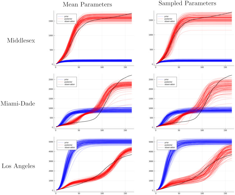
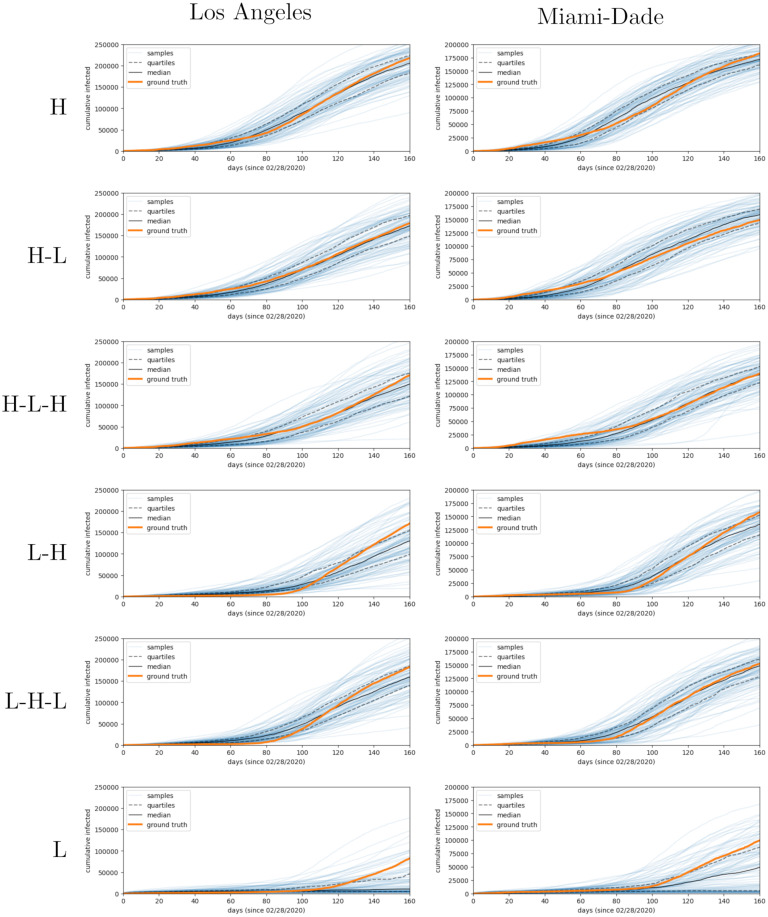
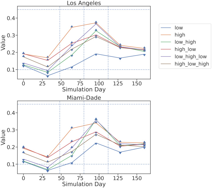
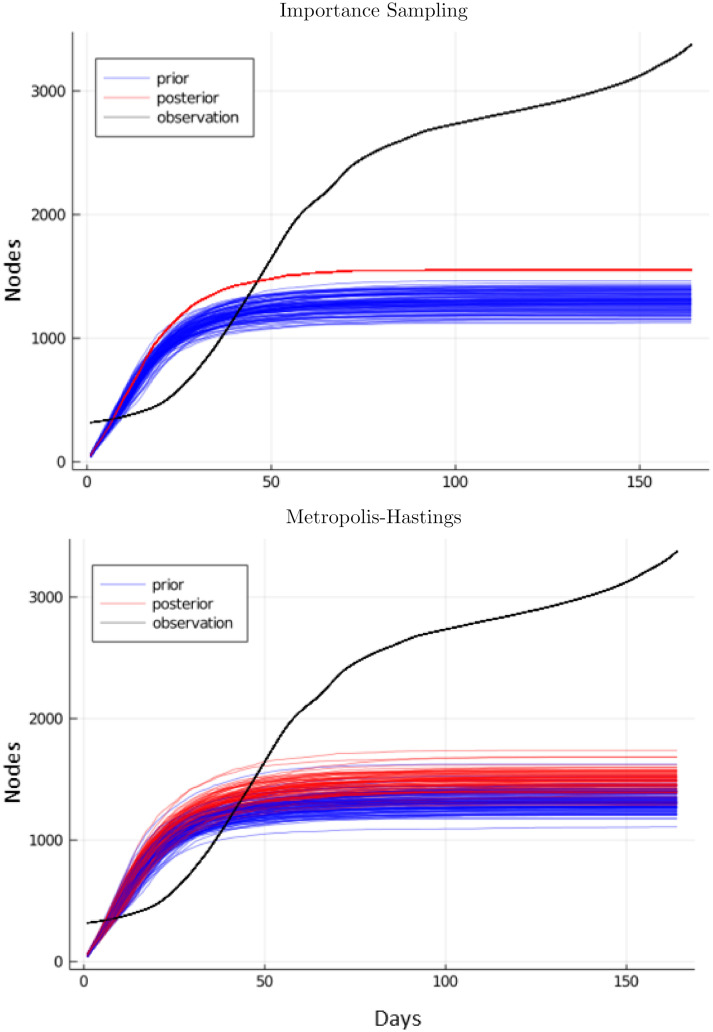
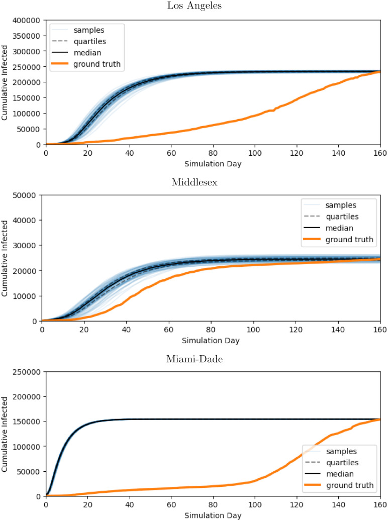
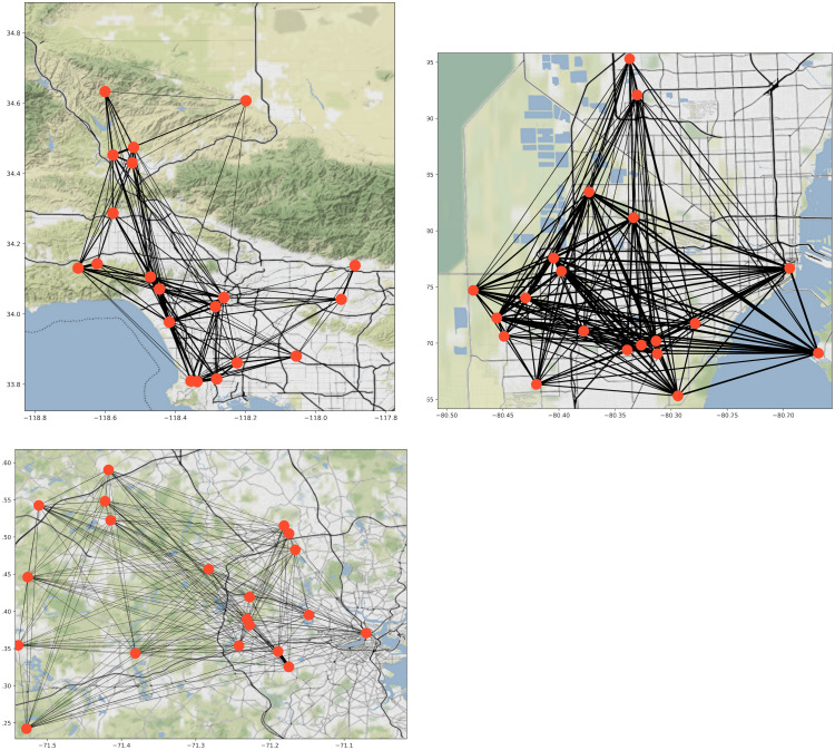
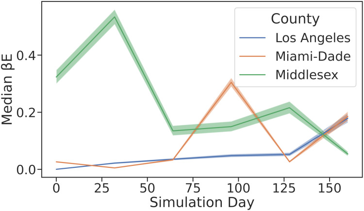
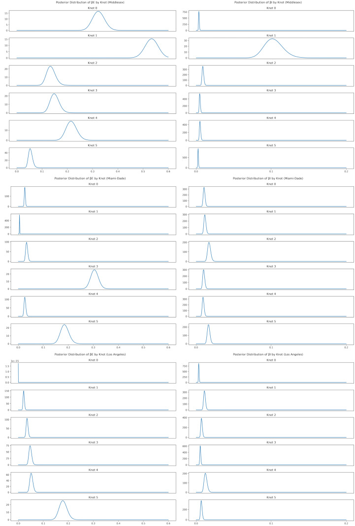
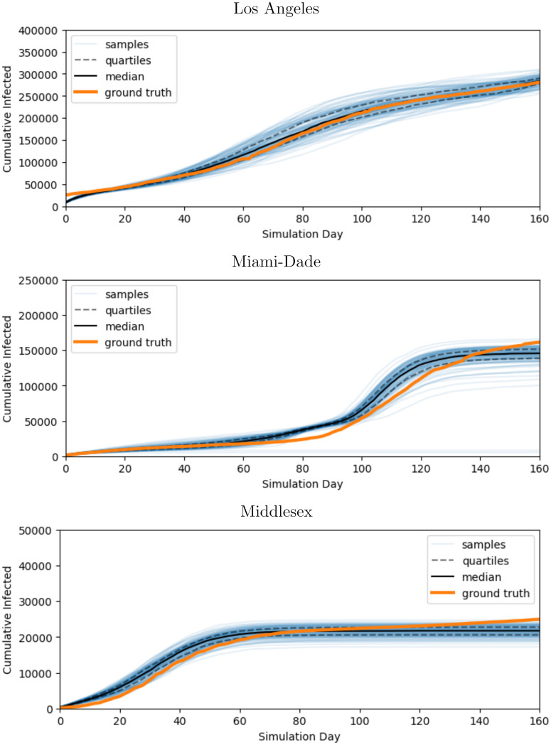
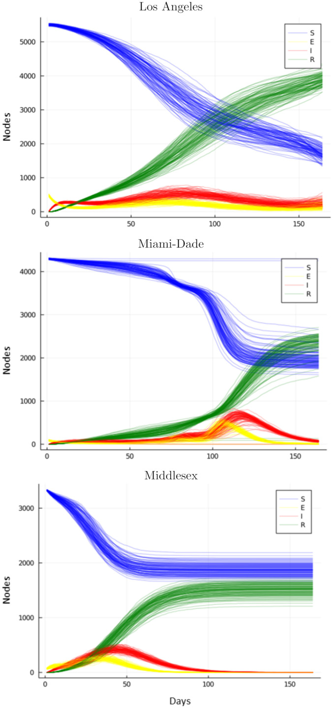
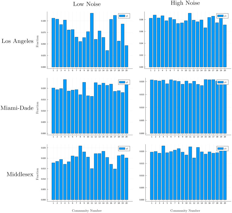
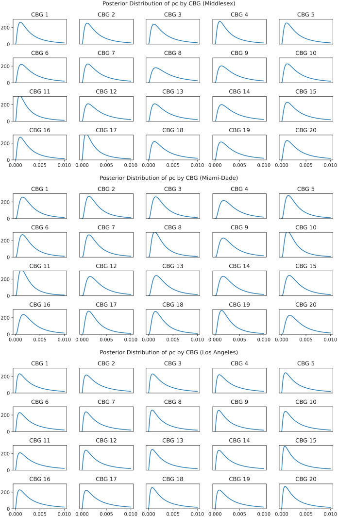
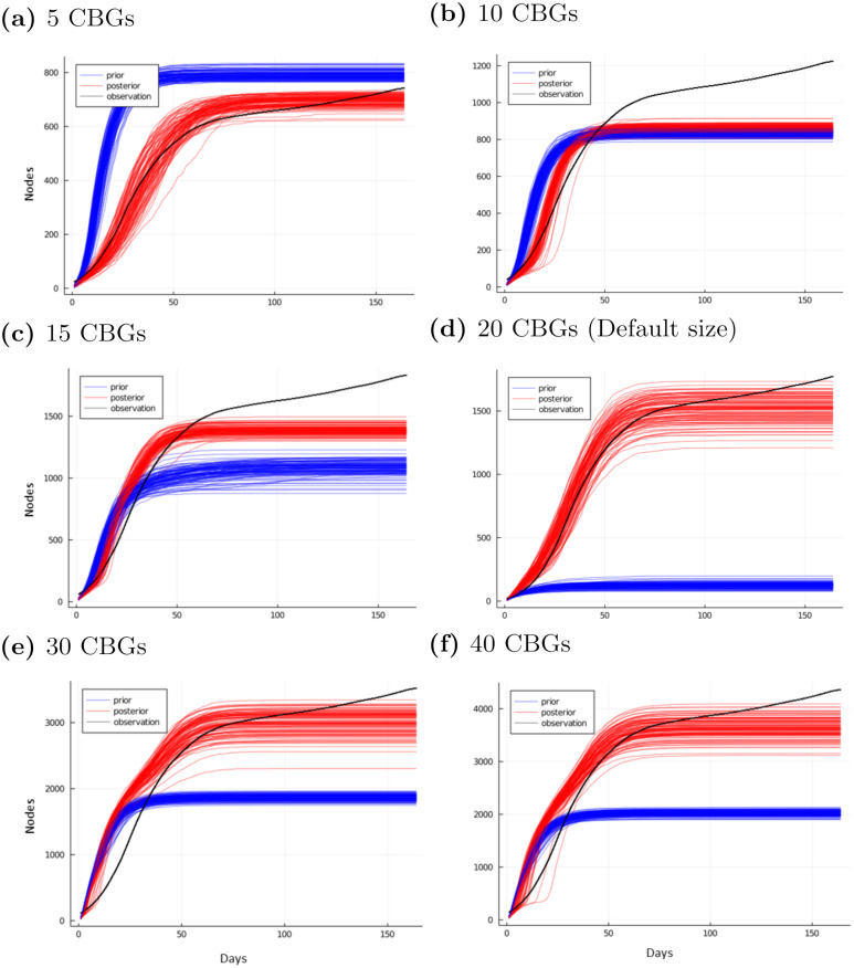
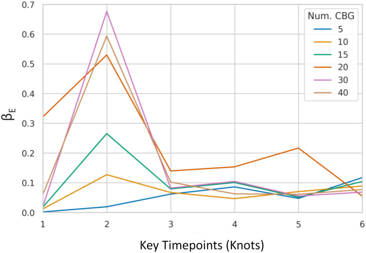
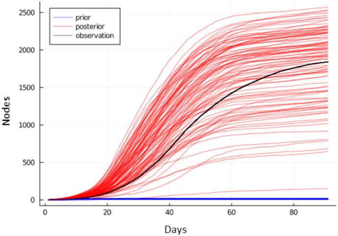
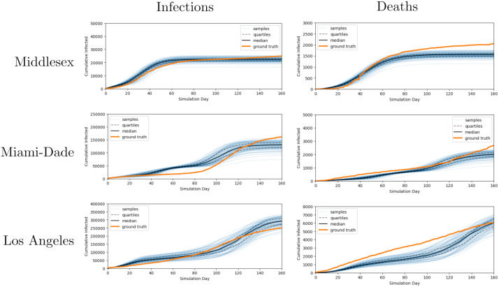
Accurate epidemiological models require parameter estimates that account for mobility patterns and social network structure. We demonstrate the effectiveness of probabilistic programming for parameter inference in these models. We consider an agent-based simulation that represents mobility networks as degree-corrected stochastic block models, whose parameters we estimate from cell phone co-location data. We then use probabilistic program inference methods to approximate the distribution over disease transmission parameters conditioned on reported cases and deaths. Our experiments demonstrate that the resulting models improve the quality of fit in multiple geographies relative to baselines that do not model network topology.

Fig 1. Cumulative infection trajectories using fixed or sampled disease parameters.

After fitting the parameters of our model to data, we show the cumulative infections produced by 100 runs of the simulator using selected parameters. On the left, we use the posterior mean parameters; the observed variation comes from the untraced randomness of network simulator. On the right, we use samples from the posterior distribution; variation comes from both the untraced randomness and the variance of our posterior distribution.

Fig 2. Sampled infection trajectories after fitting parameters on synthetic data.

We generate simulated data on Los Angeles and Miami-Dade topologies using known disease parameters, and use this data for parameter inference. Generated disease trajectories use “high”, “high-low”, “high-low-high”, “low-high”, “low-high-low”, “low” patterns, where data is simulated with β^E that varies temporally between “high” (β^E = 0.45) and “low” (β^E = 0.1) states.

Fig 3. Inferred parameter values from synthetic data.

We plot the inferred values of ${\beta }_t^E$ across 6 different generated scenarios using 6 lines. The scenarios are “high”, “high-low”, “high-low-high”, “low-high”, “low-high -low”, and “low” where β^E varies temporally between “high” β^E = 0.45 and “low” β^E = 0.1 states, represented by horizontal dotted lines. The vertical dotted lines represents the times when the true parameters were changed while generating data. The value of β used when generating the data is indicated by marker with up arrows indicating high and down arrows indicating low. We see that when the high value for β was used to generate data, the inferred value was higher and similarly the inferred value was low when the generating value was low. The inferred value for β^E is closer to the prior value of 0.2 in all scenarios at the end of the simulation when the signal from the cumulative infection counts is weaker.

Fig 4. Samples for the NSEIR model for Miami-Dade using parameters learned from likelihood weighting and Metropolis-Hastings.

Neither alternate method is able to produce a good fit.

Fig 5. R_t-analytic parameter inference baseline.

R_t-analytic derived parameters can only produce a distinctive curve shape; while this fits well for some data (such as Middlesex County above), it fits poorly much of the time.

Fig 6. Map overlay of network topologies.

Nodes from each CBG are grouped together and placed on the central coordinates for that community. Edges between CBGs represent the sum of all connected edge weights, where darker lines indicate a greater sum of edge weights. Underlying map tiles from Stamen Design under CC BY 3.0. Data by OpenStreetMap, under ODbL [53] (Top left—Los Angeles: http://maps.stamen.com/terrain-background/#10/34.0692/-118.2438. Top right—Miami-Dade: http://maps.stamen.com/terrain-background/#11/25.9046/-80.3070, Bottom—Middlesex: http://maps.stamen.com/terrain-background/#12/42.4205/-71.4415.

Fig 7. Median values of βEt from inferred distribution over time time.

Values are interpolated between 6 knots. Our inferred parameters vary over time to match the regional case counts; for example, in Middlesex county, our model infers high early values for β_E due to an early spike in regional case counts.

Fig 8. Posterior distribution of βEtn and βItn at each change point during simulation.

Fig 9. Cumulative infection trajectories sampled from fitted model.

Our method is capable of obtaining distributions of disease parameters which reproduce true data closely over a variety of regions. The orange line represents true cumulative infections counts for 160 days starting from 7 days before the first day in which infections counts accounted for 0.5% of the population: May 3, 2020 for Los Angeles, March 29, 2020 for Miami-Dade, and March 15, 2020 for Middlesex. The blue lines represent 100 simulations of f_nseir using disease parameters sampled from our fit variational distribution. The black lines represent quartiles for these 100 samples.

Fig 10. SEIR curves produced by fitted model.

Our method is capable of fitting different disease dynamics in different regions including infections with multiple waves and different rates of infectivity over time. We plot the total Susceptible, Exposed, Infected, and Removed (SEIR) counts over 160 days from 100 simulations for our fit posterior distribution.

Fig 11. Varying observation noise level controls sparsity of inferred starting conditions.

As noise distribution tightens, inference moves further from our uniform prior on initial community exposure rates. Low noise corresponds to ν = 0.00025, and high noise to ν = 0.0005. The network topology of each county is modeled using 20 communities which correspond to actual geographic areas. We plot ${\mu }_c^{\rho }$ for 1 ≤ c ≤ 20. In the left plots, we use ν = 0.00025, a tighter observational noise than the right plots where ν = 0.0005.

Fig 12. Posterior distribution of ρ_c for communities and βIt at each change point during simulation.

Note that CBGs have no correspondence across counties.

Fig 13. Prior and posterior disease trajectories with varying network size.

Applying the same prior parameters on graphs subsampled to a different initial set of CBGs produces substantially different prior behavior for the disease simulator (blue). Our inference converges to a consistent behavior (red) that is close to the observed data (black).

Fig 14. Posterior mean parameter values with varying network size.

We vary the size of our simulated network by varying the number of Census Block Groups (CBG) used during construction. We observe that the inferred disease parameters follow a similar trend even across large differences in network size.

Fig 15. Inferred cumulative infection statistics and SEIR curves for network modeled with time-varying edge weights.

Our model still finds parameters that approximately match the data, even when the network topology changes over time. Note that the model also compensates for the poor performance of the prior parameters.

Fig 16. Cumulative infection trajectories sampled from model fit to infection and death data.

We see that posterior samples of cumulative infection and death counts from several counties are generally in good agreement with the data when we use both infections and deaths as input observations to our model.

Fig 17. Convergence curves, showing the ELBO at each iteration of optimization.

We see that parameter inference has converged within the allocated computation budget.

References

1. Kermack WO, McKendrick AG. A Contribution to the Mathematical Theory of Epidemics. Proceedings of the Royal Society of London Series A, Containing papers of a mathematical and physical character. 1927;115(772):700–721.
1. Diekmann O, Heesterbeek JAP. Mathematical Epidemiology of Infectious Diseases: Model Building, Analysis and Interpretation. vol. 5. New York City: John Wiley & Sons; 2000.
1. Chinazzi M, Davis JT, Ajelli M, Gioannini C, Litvinova M, Merler S, et al.. The Effect of Travel Restrictions on the Spread of the 2019 Novel Coronavirus (COVID-19) Outbreak. Science. 2020;368(6489):395–400. doi: 10.1126/science.aba9757 - DOI - PMC - PubMed
1. Chang S, Pierson E, Koh PW, Gerardin J, Redbird B, Grusky D, et al.. Mobility Network Models of COVID-19 explain Inequities and Inform Reopening. Nature. 2021;589(7840):82–87. doi: 10.1038/s41586-020-2923-3 - DOI - PubMed
1. Grefenstette JJ, Brown ST, Rosenfeld R, DePasse J, Stone NTB, Cooley PC, et al.. FRED (a Framework for Reconstructing Epidemic Dynamics): An Open-Source Software System for Modeling Infectious Diseases and Control Strategies Using Census-Based Populations. BMC public health. 2013;13:940. doi: 10.1186/1471-2458-13-940 - DOI - PMC - PubMed
Publication types