Meta-Analysis
. 2022 Nov 7;13(1):6712.
doi: 10.1038/s41467-022-33628-8.

Discerning asthma endotypes through comorbidity mapping

Affiliations
Meta-Analysis

Discerning asthma endotypes through comorbidity mapping

Gengjie Jia et al. Nat Commun. .

Abstract

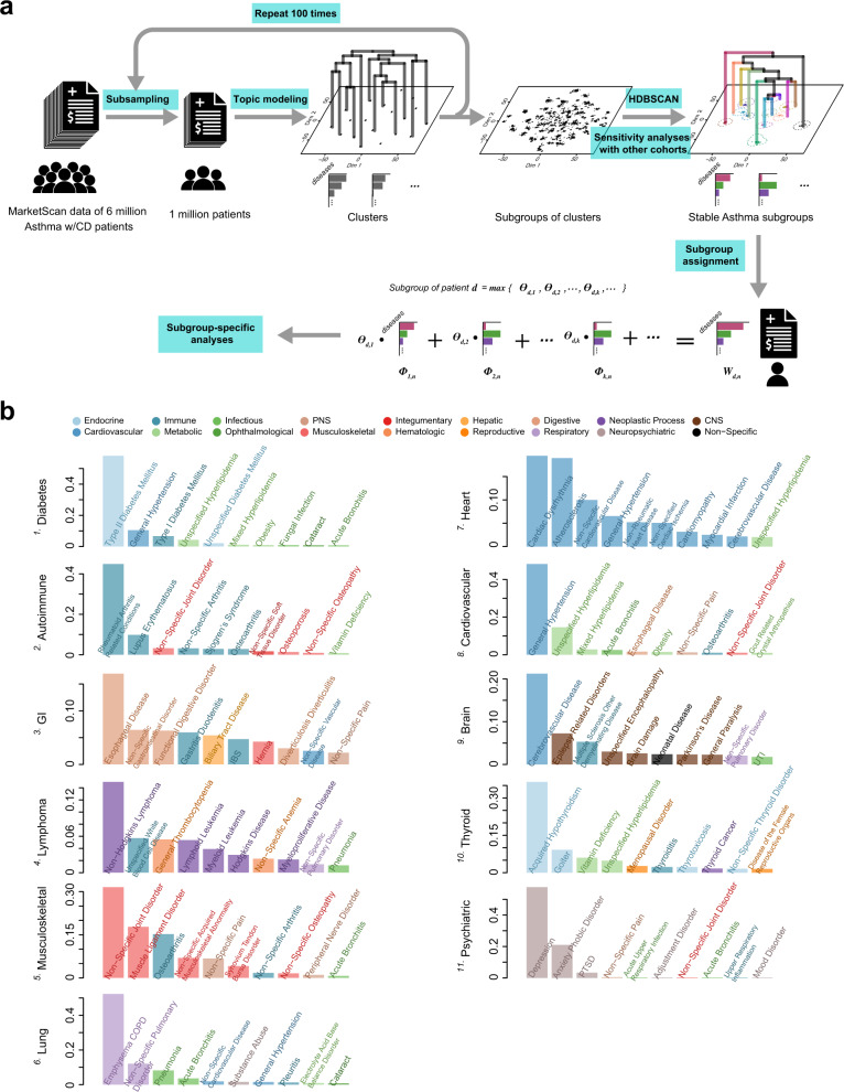
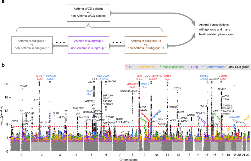
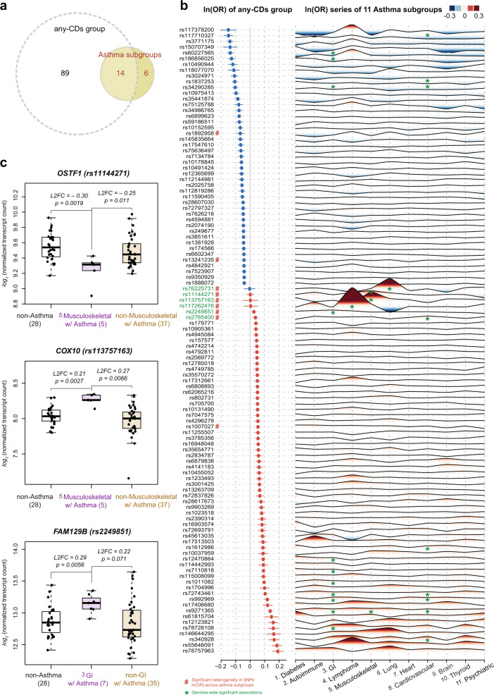
Asthma is a heterogeneous, complex syndrome, and identifying asthma endotypes has been challenging. We hypothesize that distinct endotypes of asthma arise in disparate genetic variation and life-time environmental exposure backgrounds, and that disease comorbidity patterns serve as a surrogate for such genetic and exposure variations. Here, we computationally discover 22 distinct comorbid disease patterns among individuals with asthma (asthma comorbidity subgroups) using diagnosis records for >151 M US residents, and re-identify 11 of the 22 subgroups in the much smaller UK Biobank. GWASs to discern asthma risk loci for individuals within each subgroup and in all subgroups combined reveal 109 independent risk loci, of which 52 are replicated in multi-ancestry meta-analysis across different ethnicity subsamples in UK Biobank, US BioVU, and BioBank Japan. Fourteen loci confer asthma risk in multiple subgroups and in all subgroups combined. Importantly, another six loci confer asthma risk in only one subgroup. The strength of association between asthma and each of 44 health-related phenotypes also varies dramatically across subgroups. This work reveals subpopulations of asthma patients distinguished by comorbidity patterns, asthma risk loci, gene expression, and health-related phenotypes, and so reveals different asthma endotypes.


Conflict of interest statement

J.S. reports grants from NIH, during the conduct of the study; grants from NIH, personal fees from PulmOne Advanced Medical Devices, Ltd, Israel, personal fees and non-financial support from Regeneron/Sanofi-Genzyme, grants from Chicago Biomedical Consortium Accelerator Network, outside the submitted work; in addition, J.S. has US Patents #6,090,618, #6,114,311, #6,284,743, #6,291,211, #6,297,221, #6,331,527, #7,169,764 issued, and two patent applications (WO2020206109 and WO2020206118) pending. The other authors declare no competing interests. S.W. reports grants from NIH during the conduct of the study; grants from NIH and personal fees from Regeneron/Sanofi-Genzyme and Astra-Zeneca, outside the submitted work.

Figures

Fig. 1
Fig. 1. Identification of asthma subgroups through topic modeling.
a Flowchart of asthma subgroup identification. The MarketScan data includes around six million asthma patients who have at least one comorbid disease (CD). To enable the estimation of sample statistics, we randomly selected one million patients and applied topic modeling to obtain comorbidity clusters (one cluster is projected as one point in the t-SNE plot). This procedure was repeated 100 times, generating a large collection of clusters shown as thousands of scattered points in the t-SNE projection. We used this t-SNE low-dimensional projection of topics only for visualization purpose, rather than for cluster discovery. With inter-cluster dissimilarity measured by Jensen-Shannon divergence, we applied HDBSCAN to identify stable subgroups of clusters as well as their hierarchies. A potential subgroup was deemed to be a stable “asthma subgroup”, only if it harbored more than 50 cluster points. We also conducted a sensitivity analysis on our identification approach in four additional cohorts, and subsequentially show the eleven subgroups that were commonly found in all the different cohorts above. Then, given the distribution of diagnosis counts shown in an individual’s record, we can express it as a linear combination of the distributions of diagnosis counts as defined in the asthma subgroups, and suggest that the subgroup with the largest assigned coefficient could represent the individual’s record best, therefore “assigning” the individual to this subgroup (Wd,n, Φk,n, and Θd,k contain the information about record-diagnosis co-occurrences, subgroup profiles, and assignment coefficients, respectively; see Methods for more details). b The top ten frequently occurring diseases in the identified eleven asthma subgroups. A complete and precise definition of an asthma subgroup requires one to specify the frequency distribution of 567 disease groups. For each subgroup, we use a bar plot to show its top ten frequently occurring diseases, and color-code the bars as well as the annotations by the broader categories that the diseases belong to. The y axis denotes the normalized occurring frequency of a given disease, and we can see that a subgroup is named after the broader category to which several most frequently occurring diseases belong (see Supplementary Data 1 for the subgroup profiles in detail).
Fig. 2
Fig. 2. Genome-wide significant associations with asthma.
a Study design for association analyses. Starting with the general population who may have any comorbid diseases (the any-CDs group) in UK Biobank, we were able to assign an individual with 1 of the 11 asthma subgroups that were found in UK Biobank. Then, we performed GWASs to identify asthma risk loci for the any-CDs group and for each subgroup individually (by comparing asthma cases against non-asthma controls within each subgroup). b GWAS Manhattan plots. This figure overlays GWAS results from the any-CDs group (in black) and from five selected subgroups (in multi-colors) that contained genome-wide significant asthma risk loci, including subgroups 3 “GI,” 4 “Lymphoma,” 5 “Musculoskeletal,” 6 “Lung,” and 8 “Cardiovascular.” All the association p values are shown on a –log10 scale on the y axis, and genomic locations are shown on the x-axis. The threshold of genome-wide significance (5 × 10−8) is indicated as a horizontal dashed line in red. Triangles at top indicate SNPs that have a higher –log10(p value) than shown. In addition, we annotate genome-wide significant loci with the names of their nearest genes, and in the case where a gene is commonly found in multiple subgroups and in the any-CDs group, the subgroup serial numbers and letter “G” are written, respectively, in parentheses under the gene name. In particular, we highlight the genes nearest to the six subgroup-specific loci by rotating their names with an angle of 45 degrees. More details can be found in Supplementary Table 1.
Fig. 3
Fig. 3. Summary of genome-wide significant loci and differential gene expression.
a A summary of the significant loci in a Venn diagram. The association analysis by comparing asthma cases and non-asthma controls in the any-CDs group identified 103 independent loci at genome-wide significance level. Similar association analyses within each of the eleven asthma subgroups discovered 20 significant loci, of which 14 were also seen in the any-CDs group, and, interestingly, six more loci were specific to one subgroup only. Altogether there were 109 independent loci identified. b Association results for significant loci. The forest plot on the left side summarizes the association results seen in the any-CDs group for the 109 loci, at which the lead SNPs are listed in the first column. Squares denote the effect sizes, i.e., natural logarithm of odds ratios or ln(OR), and horizontal lines are the 95% confidence intervals. From top to bottom, the effect sizes are in ascending order, from negative (in blue) to positive values (in red). The wave-like plot on the right side displays a series of effect sizes seen in the eleven subgroups that can be found in UK Biobank for each of the 109 SNPs. The subgroup names are labeled along the horizontal axis, while for each of the 109 SNPs that are displayed along the vertical axis, its effect size is represented as a peak in the red shade if it is positive, and as a trough in blue shade if negative. The absolute value of the effect size is proportional to the height (or depth) of the peak (or trough), and is also color-coded. All the genome-wide significant associations between SNPs and subgroups are marked with green asterisks, and in particular, the six SNPs that are specific to one subgroup only are highlighted in green in the first name column. In addition, the heterogeneity of per-locus effect sizes across the eleven subgroups was assessed through a Cochran’s Q test, finding nine loci with evidence of significant heterogeneity in effect sizes (indicated with # symbols in red after the respective SNP names in the first column). See Supplementary Data 6 for the association results in detail and Supplementary Fig. 5 for the numbers of allocated cases and controls in each subgroup. c Differential gene expression. For three of the subgroup-specific SNPs, we confirmed the differential expression of their nearby genes (i.e., OSTF1, COX10, and FAM129B), using an independent dataset of bronchial epithelial transcriptome profiles. The gene OSTF1, for example, has significantly lower expression among asthma cases in subgroup 5 “Musculoskeletal”, compared to non-asthma controls and asthma cases in other subgroups (see the x axis labels and respective sample sizes in parentheses). The y-axis shows the normalized transcript count on a log2 scale, i.e., log2[(transcript count+0.5)/size factor]; the minimum, the first quartile, the median, the third quartile, and the maximum of OSTF1 for non-asthma controls are 9.17, 9.42, 9.54, 9.67, and 9.93, for asthma cases in subgroup 5 are 8.91, 9.24, 9.31, 9.34, and 9.43, and for asthma cases in other subgroups are 9.20, 9.34, 9.45, 9.59, and 9.97; these values of COX10 for non-asthma controls are 7.80, 7.97, 8.03, 8.12, and 8.30, for asthma cases in subgroup 5 are 8.14, 8.26, 8.26, 8.33, and 8.35, and for asthma cases in other subgroups are 7.15, 7.86, 8.00, 8.09, and 8.33; these values of FAM129B for non-asthma controls are 12.41, 12.71, 12.85, 13.01, and 13.44, for asthma cases in subgroup 3 are 12.91, 13.06, 13.15, 13.23, and 13.35, and for asthma cases in other subgroups are 12.28, 12.62, 12.73, 13.04, and 13.64). The mean log2 fold changes (L2FC) of OSTF1 in subgroup 5 of asthma cases were −0.30 (two-sided Wald statistic p value = 0.0019) and −0.25 (p value = 0.011), when compared to non-asthma controls and asthma cases in other subgroups, respectively. The other comparisons show that bronchial epithelial cell expression of COX10 in subgroup 5 “Musculoskeletal” and FAM129B in subgroup 3 “GI” are significantly higher, compared to non-asthma controls and their respective asthma cases in other subgroups.
Fig. 4
Fig. 4. Differential asthma associations with health-related phenotypes across subgroups.
A total of 10 different categories of health-related phenotypes (140 different measurements in total) were subjected to phenotype association analysis (see Methods for technical details and Supplementary Data 11 for the numbers of allocated cases and controls in each subgroup). We first computed phenotypes’ slope estimates of asthma associations within each subgroup and in the any-CDs group. The direction and strength of the association are characterized by the sign and absolute value of the slope, respectively. a Heterogeneous slope estimates related to blood count. We assessed the heterogeneity in these slope estimates across subgroups for each phenotype, and benchmarked against the slope value for that phenotype in the any-CDs group. Each phenotype is presented as a meta-plot, which shows the posterior means (as squares) and 95 percent confidence intervals (as error bars) of the slopes from subgroups 1 to 11 that were also discovered in UK Biobank (displayed from top to bottom). Slope estimates that are significantly less positive than the any-CDs group benchmark (marked by a vertical dashed line) are shown in blue, while those that are significantly more positive are shown in red; the respective subgroup numbers are also shown for significantly different subgroups. For example, subgroup 6 “Lung” exhibits many red-blood-cell-related phenotypes that are in significantly stronger associations with asthma likelihood than appear for the general population in the any-CDs group. b Heterogeneous slope estimates related to the local environment, diet, and physical activity. In the same fashion as shown in a, we display the meta-plots of the phenotypes in the categories of the local environment, diet, and physical activity. A distinct pattern of these phenotypes distinguishes subgroup 1 “Diabetes,” in which stronger associations of greenspace, air quality, salt intake, and exercise are evident.

References

    1. CDC.gov. CDC - Asthma - Data and Surveillance - Asthma Surveillance Data. Available at: http://www.cdc.gov/asthma/asthmadata.htm [Accessed 15 September 2019] (2018).
    1. Woodruff PG, et al. Genome-wide profiling identifies epithelial cell genes associated with asthma and with treatment response to corticosteroids. Proc. Natl Acad. Sci. USA. 2007;104:15858–15863. - PMC - PubMed
    1. Bouzigon E, et al. Effect of 17q21 variants and smoking exposure in early-onset asthma. N. Engl. J. Med. 2008;359:1985–1994. - PubMed
    1. Haldar P, et al. Cluster analysis and clinical asthma phenotypes. Am. J. Respir. Crit. Care Med. 2008;178:218–224. - PMC - PubMed
    1. Dweik RA, et al. Use of exhaled nitric oxide measurement to identify a reactive, at-risk phenotype among patients with asthma. Am. J. Respir. Crit. Care Med. 2010;181:1033–1041. - PMC - PubMed

Publication types