Machine learning-based detection of label-free cancer stem-like cell fate

Abstract

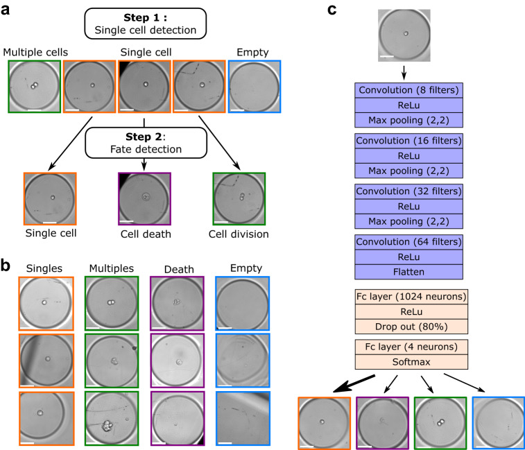
The detection of cancer stem-like cells (CSCs) is mainly based on molecular markers or functional tests giving a posteriori results. Therefore label-free and real-time detection of single CSCs remains a difficult challenge. The recent development of microfluidics has made it possible to perform high-throughput single cell imaging under controlled conditions and geometries. Such a throughput requires adapted image analysis pipelines while providing the necessary amount of data for the development of machine-learning algorithms. In this paper, we provide a data-driven study to assess the complexity of brightfield time-lapses to monitor the fate of isolated cancer stem-like cells in non-adherent conditions. We combined for the first time individual cell fate and cell state temporality analysis in a unique algorithm. We show that with our experimental system and on two different primary cell lines our optimized deep learning based algorithm outperforms classical computer vision and shallow learning-based algorithms in terms of accuracy while being faster than cutting-edge convolutional neural network (CNNs). With this study, we show that tailoring our deep learning-based algorithm to the image analysis problem yields better results than pre-trained models. As a result, such a rapid and accurate CNN is compatible with the rise of high-throughput data generation and opens the door to on-the-fly CSC fate analysis.

Figure 1

Description of our deep-learning based algorithm (DLBA). (a) Visual abstract of the image analysis problem. First step: detection of isolated single cells from 2D brightfield images. Second step: when a single cell was detected, the 96-h time-lapse of the corresponding well was analysed in order to detect cell division or cell death. (b) Examples of the different classes defined for our DLBA: single cells, multiple cells, dead cells or empty well. (c) Model of our optimized DLBA : 4 convolution layers before classification of images between “Singles”, “Multiples”, “Death” and “Empty”. Scale bar: 50 $\mathrm{\mu }$m.

Figure 2

Working principles of the CCVA and SLBA tested in this study. (a) For the CCVA, images were processed through an intensity threshold before a size filtering. Remaining objects were fit to an ellipse. First row: processing of a well containing a single cell, second row: processing of a well containing multiple cells. (b) According to the area and roundness of the ellipse, images were classified as “Singles”, “Multiples”, “Death” or “Empty”. (c) For the SLBA, the first step of pixel classification segments cells from the background. Then, thanks to an object classification tool (Ilastik), images were classified between “Singles”, “Multiples”, “Death” and “Empty” categories. The first row shows the processing of an image classified as “Single”, second row image of well classified as “Multiple”. Colour code corresponds to Fig. 1. Scale bars show 50 μm.

Figure 3

Global accuracy comparison between the different methods tested. (a) For our optimized DLBA: Double entry table analysing differences between the ground truth (“True label”, vertical axis) and the prediction (“Predicted label”, horizontal axis). Our optimized DLBA provided an accuracy of $91.2\pm 0.17\%$. Recall and precision were respectively 87% and 81% for “Singles”, 90% and 93% for “Multiple”, 70% and 42% for “Death”, and 91% and 97% for “Empty”. (b) The CCVA provided an accuracy of 65%. Recall and precision were respectively 22% and 66% for “Singles”, 42% and 62% for “Multiple”, 1% and 3% for “Death”, and 89% and 63% for “Empty”. (c) The SLBA provided an accuracy of 72%. Recall and precision were respectively 51% and 55% for “Singles”, 64% and 81% for “Multiple”, 22% and 10% for “Death”, and 88% and 85% for “Empty”. The color range stands for the amount of images in each category: the darker, the more images are associated. (d) Accuracy versus computation times for the 7 methods tested, for 1000 images See Table 1.

Figure 4

Dynamic analysis with our DLBA. (a) Downstream of the CNN, a decision tree considers the temporal information of cell time-lapses in order to detect single cells, cell divisions and cell death. First, we performed a majority voting on the first three frames for each microwell. If all these three frames were classified as “Empty”, the microwell was considered as containing no cell and its time-lapse was not further analysed. Then, if any of these three first frames was classified as “Multiple” or “Death”, the microwell was respectively considered as containing multiple cells or dead cells and was discarded from further analysis too. Finally, if all the three first frames were classified as “Single”, the microwell was considered as containing a single cell and the analysis kept on going. Among each time-lapse with an initial single cell, if two frames were classified as “Multiple” with a probability> 0.9 (of which one>0.99), we considered that a cell division occurred in the microwell. Else, if any frame was classified as “Death” with a >0.5 probability, we considered that a cell death occurred in the microwell. In any other case, we considered that there were still a living yet non-dividing cell in the microwell. (b) Examples of Time-Lapse images displaying cell division, death or neither of the two. Scale bars: 50 $\mu$M. Cumulative dynamics of N14-0510 cells divisions (c) and cell death (e) were computed over time. Relative division rate (d) and death rate (f) were computed, over sliding 6-h temporal windows. Plots show means and standard deviations, over 4 experiments with three replicates each (2780 time-lapses analyzed in total).

References

1. Dirkse A, et al. Stem cell-associated heterogeneity in Glioblastoma results from intrinsic tumor plasticity shaped by the microenvironment. Nat. Commun. 2019;10:1787. doi: 10.1038/s41467-019-09853-z. - DOI - PMC - PubMed
1. Nassar D, Blanpain C. Cancer stem cells: basic concepts and therapeutic implications. Annu. Rev. Pathol.: Mech. Dis. 2016;11:47–76. doi: 10.1146/annurev-pathol-012615-044438. - DOI - PubMed
1. Pastrana E, Silva-Vargas V, Doetsch F. Eyes wide open: a critical review of sphere-formation as an assay for stem cells. Cell Stem Cell. 2011;8:486–498. doi: 10.1016/j.stem.2011.04.007. - DOI - PMC - PubMed
1. Lathia JD, Mack SC, Mulkearns-Hubert EE, Valentim CLL, Rich JN. Cancer stem cells in glioblastoma. Genes Dev. 2015;29:1203–1217. doi: 10.1101/gad.261982.115. - DOI - PMC - PubMed
1. Icha, J., Weber, M., Waters, J. C. & Norden, C. Phototoxicity in live fluorescence microscopy, and how to avoid it. Bioessays 39, 10.1002/bies.201700003 (2017). - PubMed
Publication types