Through the looking glass: Deep interpretable dynamic directed connectivity in resting fMRI

Abstract

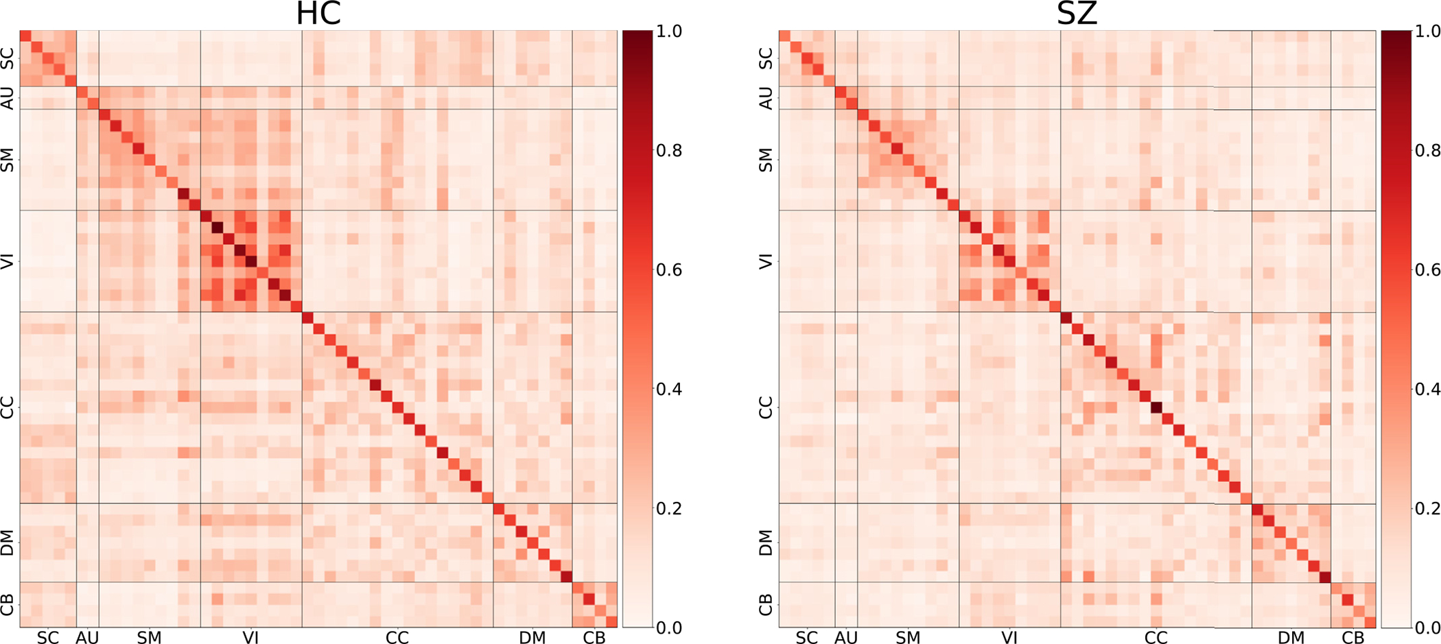
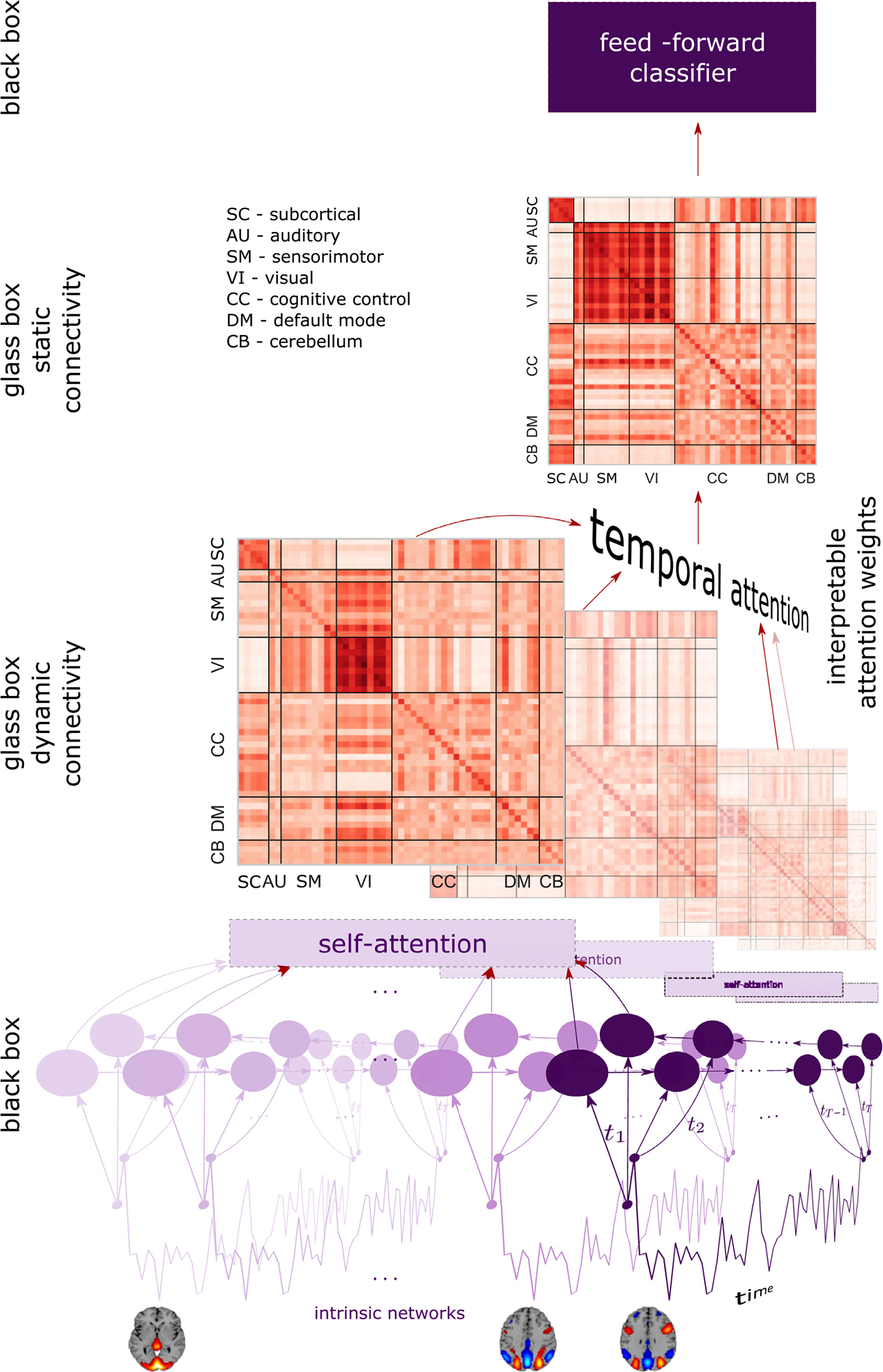
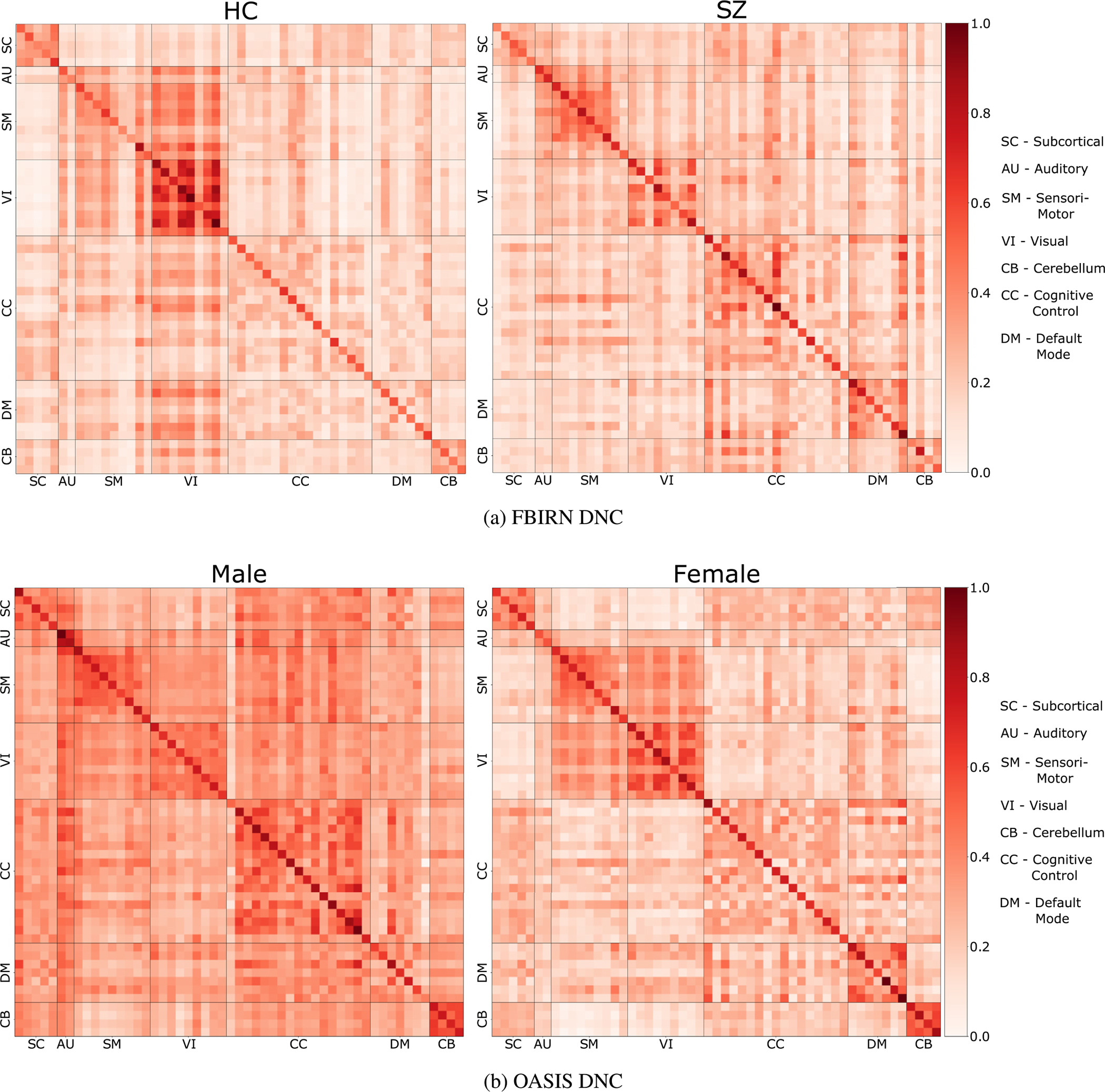
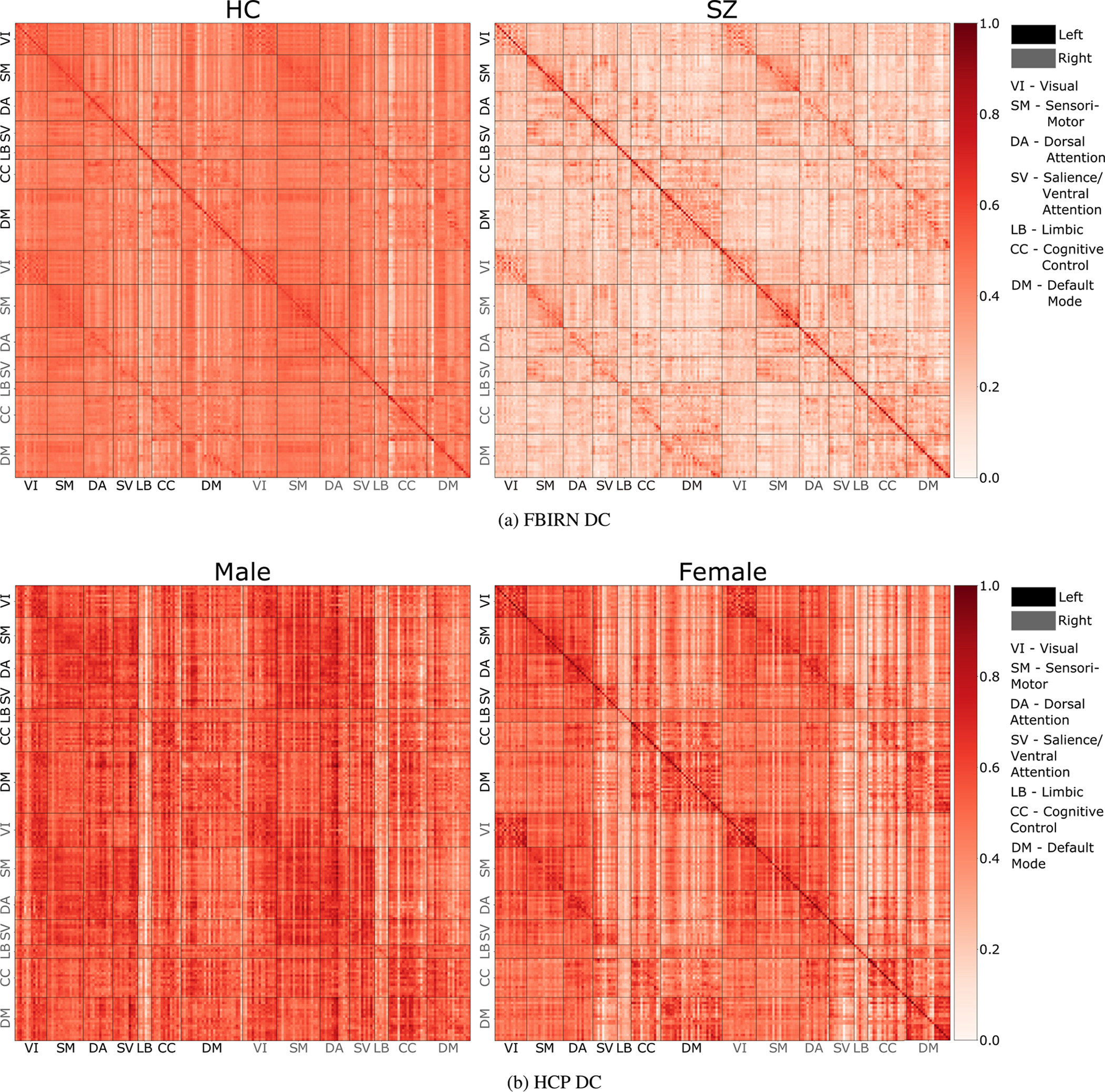
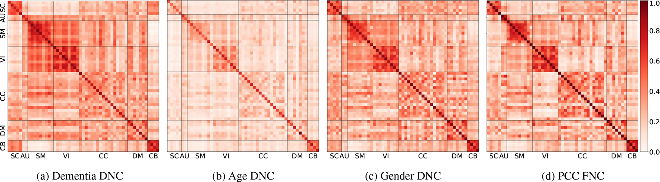
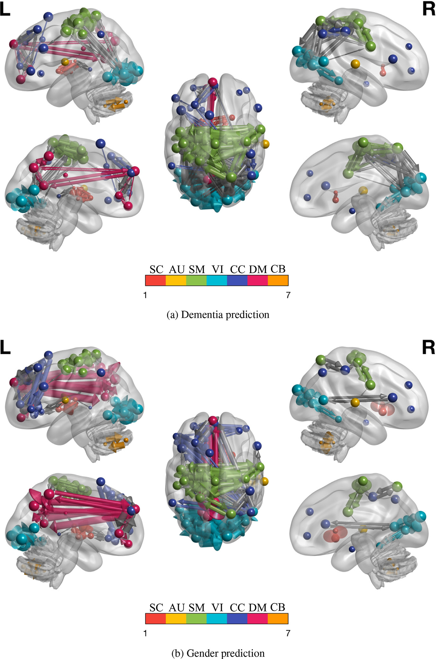
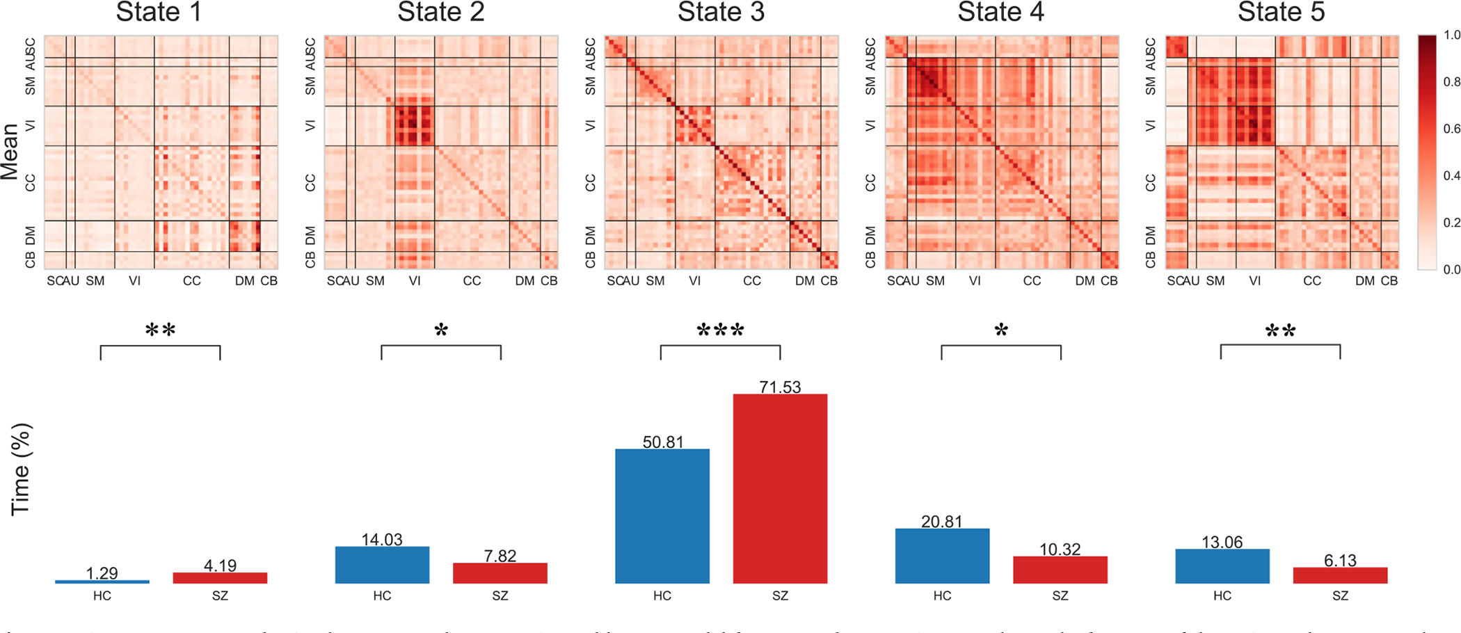
Brain network interactions are commonly assessed via functional (network) connectivity, captured as an undirected matrix of Pearson correlation coefficients. Functional connectivity can represent static and dynamic relations, but often these are modeled using a fixed choice for the data window Alternatively, deep learning models may flexibly learn various representations from the same data based on the model architecture and the training task. However, the representations produced by deep learning models are often difficult to interpret and require additional posthoc methods, e.g., saliency maps. In this work, we integrate the strengths of deep learning and functional connectivity methods while also mitigating their weaknesses. With interpretability in mind, we present a deep learning architecture that exposes a directed graph layer that represents what the model has learned about relevant brain connectivity. A surprising benefit of this architectural interpretability is significantly improved accuracy in discriminating controls and patients with schizophrenia, autism, and dementia, as well as age and gender prediction from functional MRI data. We also resolve the window size selection problem for dynamic directed connectivity estimation as we estimate windowing functions from the data, capturing what is needed to estimate the graph at each time-point. We demonstrate efficacy of our method in comparison with multiple existing models that focus on classification accuracy, unlike our interpretability-focused architecture. Using the same data but training different models on their own discriminative tasks we are able to estimate task-specific directed connectivity matrices for each subject. Results show that the proposed approach is also more robust to confounding factors compared to standard dynamic functional connectivity models. The dynamic patterns captured by our model are naturally interpretable since they highlight the intervals in the signal that are most important for the prediction. The proposed approach reveals that differences in connectivity among sensorimotor networks relative to default-mode networks are an important indicator of dementia and gender. Dysconnectivity between networks, specially sensorimotor and visual, is linked with schizophrenic patients, however schizophrenic patients show increased intra-network default-mode connectivity compared to healthy controls. Sensorimotor connectivity was important for both dementia and schizophrenia prediction, but schizophrenia is more related to dysconnectivity between networks whereas, dementia bio-markers were mostly intra-network connectivity.

Keywords: Brain disorders; Dynamic directed connectivity; Interpretable deep learning; Resting state fMRI.

Fig. B1.

DNC estimated by DICE model using the loss Eq. (B.1). We used the same FBIRN subjects as in Fig. 6a.

Fig. B2.

Comparison of the DNCs learned with the additional regularization terms in the loss function against the DNC created using original loss and PCC FNC. As expected, regularization pushes the diagonal closer to 1. Also the difference between values of diagonal and non-diagonal elements is higher in tanh based DNC B.14 b as compared to sigmoid based DNC B.14 c. Similarly to Fig. 4 these matrices are averaged across multiple tries.

Fig. B3.

DNC estimated by DICE model by incorporating negative weights in self-attention module. We used the same FBIRN subjects as in Fig. 4a. The diagonal is manually assigned 0 weight.

Fig. 1.

DICE architecture using biLSTM, self-attention and temporal attention. We use self-attention between the embeddings of all components/nodes at each time-point to estimate the DC W_i. Temporal attention is used to create a weighted sum of the T DC. Architecture details of temporal attention is shown in Fig. 2.

Fig. 2.

GTA architecture for temporal attention. W_1−T matrices are summed to create W^global. Using W^global and W_i attention score α_i is created for each time-point. Refer to equations in 3 and 4 for working details. Here f denotes the average function.

Fig. 3.

AUC comparision of DICE model with four different methods (MILC Mahmood et al. (2020), STDIM Mahmood et al. (2019), logistic regression (LR), support vector machine (SVM)), over four different datasets using ICA time-courses (Ref to Section 2.1.1). Our method significantly outperforms SOTA methods. We performed Autism experiments with 869 subjects (all TRs) as well. As we do not have a pre-training step we compare with not-pre-trained (NPT) version of MILC and STDIM. Input to ML methods were the same ICA time-courses, not the FNC matrices. We did not find any notable studies for gender classification of HCP subjects using ICA components as notable methods used ROIs based data. We compare the results using ROIs in Table 2.

Fig. 4.

We compare our estimated DNC with computed FNC using PCC method. 4 a is the connectivity matrix generated by our model for FBIRN dataset. We used a test fold of 16 subjects and computed mean FNC for all subjects (10 trials per subject). 4 b is the mean connectivity matrix of the same subjects generated by PCC. Both figures show similar intra-network connectivity patterns, which verifies the correctness of the connectivity matrix learned by our model. Our estimated DC is directed and captures more inter-network connectivity than FNC. To match the positive weights of our model, we have normalized the FNC from 0 to 1 instead of −1 to 1.

Fig. 5.

We show the top 10% directed edges of FBIRN DNC. The numbers represent the 53 non-artifact components. The figure clearly shows the high intra-domain connectivity which matches the existing literature. Direction clearly matters as visual components affect other components but not the opposite way. The direction of edges between CC and SM networks is also of significance.

Fig. 6.

We compare the estimated DNC across the binary classification groups using ICA data. Figure 6a is the estimated DNC on FBIRN data for HC and SZ patients. We see high inter and intra-connectivity in SM and VI networks for HC, which is missing in SZ patients. Figure 6b compares DNC between male and female groups using OASIS data. Female group shows hyper-connectivity in DMN and hypo-connectivity in SMN when comparing to male groups.

Fig. 7.

We compare the estimated DCs of HC with SZ and male with female using region-based (ROIs) FBIRN and HCP data. 7 a show high weakly connected brain networks for SZ subjects whereas 7 b show hyper-connectivity of DMN and hypo-connectivity for SMN for females as compared to females. The black and grey color denotes the regions in left and right side of the brain. Refer to Table 7 for a statistical comparison between female and male DCs.

Fig. 8.

We show how our model estimates flexible DNC structures based on the ground-truth signal. We train our model for different classification tasks and use same test subjects to compare the estimated DNC for the subjects. All figures are mean DNC estimated for the same subjects with 5 randomly-seeded trials. 8 a is the mean connectivity matrix estimated by our model when trained to classify dementia. We see high connectivity values for SC, SM, and CB networks. 8 c is the mean DNC for the same subjects when the model is trained for gender prediction. We notice lower SM network connectivity and higher connectivity for DM network when predicting gender of OASIS subjects. 8 d is the FNC computed using PCC. The FNC is independent of the task and would remain fixed (inflexible).

Fig. 9.

We map on the brain, the nodes and top 10% edges of the DCs, estimated for dementia and gender classification tasks, performed on OASIS dataset (same subjects). The size of the nodes is the sum of the outgoing and incoming edge weights. The arrows shows the direction of connectivity. We see a high number and size of nodes and edges for SMN and VIN for dementia 9 a, whereas for gender 9 b we see high node and edge size for DMN. Compare the red (DM) nodes and edges in Fig. 9a with b in the left side figures. Figure 9a also shows high connectivity between SM and VI networks which is missing in Fig. 9b (right side figures). This reveals the networks and edges (graphs and subgraphs) relevant to the classification signal (e.g disorder) without need of comparison with other data. The results and their impact are further discussed in Section 4.3. (For interpretation of the references to colour in this figure legend, the reader is referred to the web version of this article.)

Fig. 10.

Five states computed using k-means on the DCs estimated by our model for FBIRN dataset. First row shows the k means of the estimated DCs, second row shows the percentage time spent by both groups in each state, with the total time points being 155. Time spent in each state by SZ and HC differ significantly and matches the existing literature. We see that a) time spent in each state is different by HC and SZ, b) SZ spend much more time in state 3 (weakly connected) than HC, c) HC spend more time than SZ in states (2,4, 5) which show high connectivity for VI, and SM networks, and d) Standard deviation of time for SZ is much higher (320.47) than HC (206.26) which shows that SZ stay in one state much more than HC which tend to change state more often. The stars denote the significance of difference in time spent in each state by the two groups. Table 6 shows the p-value significance ranges.

Fig. 11.

We show 10 states captured by k-means on the temporal DCs estimated by DICE on FBIRN complete dataset. The rows shows the means and the percentage of time spent by HC and SZ subjects in each state. We see that DICE can capture more states than the standard (4–5) states captured by window-based approaches. The additional states not present in Fig. 10 show the change of direction in connectivity. State 9 shows the opposite direction of connectivity between VIN and other networks, where VIN has mostly incoming edges. The ratio of time spent by HC and SZ subject in different states is similar to the results of Fig. 10.

Fig. 12.

Temporal Attention weights for one of the test folds (16 subjects) of FBIRN. Attention weights are computed using GTA module. X and y axis represent time-points and subject number respectively. We show that for each subject, the attention weights remain stable across multiple randomly-seeded trials (10). The values of the 10 trials are used to create the confidence interval for each subject. The consistency is greatly increased with an increase in number of training subjects. Note: For each subject we added the subject number to the attention weights to separate the weights, as for each subject the weights have a range of 0 – 1. Dark and light colors represent SZ and HC subjects respectively.

References

-
- Aertsen A, Preissl H, 1991. Dynamics of activity and connectivity in physiological neuronal networks. Nonlinear Dyn. Neuronal Netw 281–302.
- Albers MW, Gilmore GC, Kaye J, Murphy C, Wingfield A, Bennett DA, Boxer AL, Buchman AS, Cruickshanks KJ, Devanand DP, Duffy CJ, Gall CM, Gates GA, Granholm AC, Hensch T, Holtzer R, Hyman BT, Lin FR, Mc-Kee AC, Morris JC, Petersen RC, Silbert LC, Struble RG, Trojanowski JQ, Verghese J, Wilson DA, Xu S, Zhang LI, 2015. At the interface of sensory and motor dysfunctions and Alzheimer’s disease. Alzheimers Dement 11 (1), 70–98. [DOI: 10.1016/j.jalz.2014.04.514] - DOI - PMC - PubMed
- Allen E, Erhardt E, Damaraju E, Gruner W, Segall J, Silva R, Havlicek M, Rachakonda S, Fries J, Kalyanam R, Michael A, Caprihan A, Turner J, Eichele T, Adelsheim S, Bryan A, Bustillo J, Clark V, Feldstein Ewing S, Filbey F, Ford C, Hutchison K, Jung R, Kiehl K, Kodituwakku P, Komesu Y, Mayer A, Pearlson G, Phillips J, Sadek J, Stevens M, Teuscher U, Thoma R, Calhoun V, 2011. A baseline for the multivariate comparison of resting-state networks. Front. Syst. Neurosci. 5, 2. doi:10.3389/fnsys.2011.00002. - DOI - PMC - PubMed
Publication types
MeSH terms
Grants and funding
- R21 HL129047/HL/NHLBI NIH HHS/United States
- R01 AG043434/AG/NIA NIH HHS/United States
- R01 DA040487/DA/NIDA NIH HHS/United States
- P01 AG026276/AG/NIA NIH HHS/United States
- RF1 MH121885/MH/NIMH NIH HHS/United States
- R01 EB009352/EB/NIBIB NIH HHS/United States
- U54 MH091657/MH/NIMH NIH HHS/United States
- K23 MH087770/MH/NIMH NIH HHS/United States
- R41 MH122201/MH/NIMH NIH HHS/United States
- R01 MH129047/MH/NIMH NIH HHS/United States
- R01 EB006841/EB/NIBIB NIH HHS/United States
- P01 AG003991/AG/NIA NIH HHS/United States
- R03 MH096321/MH/NIMH NIH HHS/United States
- UL1 TR000448/TR/NCATS NIH HHS/United States
- U24 RR021992/RR/NCRR NIH HHS/United States
LinkOut - more resources
Full Text Sources